Modeling and removing unwanted technical variation
Anthony Hung
2021-01-19
Last updated: 2021-01-21
Checks: 7 0
Knit directory: invitroOA_pilot_repository/
This reproducible R Markdown analysis was created with workflowr (version 1.6.2). The Checks tab describes the reproducibility checks that were applied when the results were created. The Past versions tab lists the development history.
Great! Since the R Markdown file has been committed to the Git repository, you know the exact version of the code that produced these results.
Great job! The global environment was empty. Objects defined in the global environment can affect the analysis in your R Markdown file in unknown ways. For reproduciblity it’s best to always run the code in an empty environment.
The command set.seed(20210119) was run prior to running the code in the R Markdown file. Setting a seed ensures that any results that rely on randomness, e.g. subsampling or permutations, are reproducible.
Great job! Recording the operating system, R version, and package versions is critical for reproducibility.
Nice! There were no cached chunks for this analysis, so you can be confident that you successfully produced the results during this run.
Great job! Using relative paths to the files within your workflowr project makes it easier to run your code on other machines.
Great! You are using Git for version control. Tracking code development and connecting the code version to the results is critical for reproducibility.
The results in this page were generated with repository version 78cfbcd. See the Past versions tab to see a history of the changes made to the R Markdown and HTML files.
Note that you need to be careful to ensure that all relevant files for the analysis have been committed to Git prior to generating the results (you can use wflow_publish or wflow_git_commit). workflowr only checks the R Markdown file, but you know if there are other scripts or data files that it depends on. Below is the status of the Git repository when the results were generated:
Ignored files:
    Ignored:    .DS_Store
    Ignored:    .Rhistory
    Ignored:    .Rproj.user/
    Ignored:    data/.DS_Store
    Ignored:    data/external_scRNA/.DS_Store

Untracked files:
    Untracked:  data/filtered_counts.rds
    Untracked:  data/norm_filtered_counts.rds

Unstaged changes:
    Deleted:    analysis/figure/powerAnalysis.Rmd/curve-1.png
    Deleted:    analysis/figure/powerAnalysis.Rmd/hypoxia-1.png
    Deleted:    analysis/figure/powerAnalysis.Rmd/hypoxia-2.png
    Deleted:    analysis/figure/powerAnalysis.Rmd/hypoxia-3.png
    Deleted:    analysis/figure/powerAnalysis.Rmd/hypoxia-4.png
    Deleted:    analysis/figure/powerAnalysis.Rmd/hypoxia-5.png
    Deleted:    analysis/figure/powerAnalysis.Rmd/hypoxia-6.png
    Deleted:    analysis/figure/powerAnalysis.Rmd/hypoxia-7.png
    Deleted:    analysis/figure/powerAnalysis.Rmd/hypoxia-8.png
Note that any generated files, e.g. HTML, png, CSS, etc., are not included in this status report because it is ok for generated content to have uncommitted changes.
These are the previous versions of the repository in which changes were made to the R Markdown (analysis/removeUnwantedVariation_bulkRNA.Rmd) and HTML (docs/removeUnwantedVariation_bulkRNA.html) files. If you’ve configured a remote Git repository (see ?wflow_git_remote), click on the hyperlinks in the table below to view the files as they were in that past version.
| File | Version | Author | Date | Message |
|---|---|---|---|---|
| Rmd | e3fbd0f | Anthony Hung | 2021-01-21 | add ward et al data files to data |
| html | e3fbd0f | Anthony Hung | 2021-01-21 | add ward et al data files to data |
| Rmd | 0711682 | Anthony Hung | 2021-01-21 | start normalization file |
| Rmd | 28f57fa | Anthony Hung | 2021-01-19 | Add files for analysis |
Introduction
This code takes in the normalized and filtered count data. It first performs a PCA on the data. It then looks for correlations between the first 5 PCs and several experimental variables before and after fitting two factors of unwanted variation in the data using RUVs (taking advantage of the technical replicates in our study design). We then save the RUVs output for use in later files.
Examine normalized/filtered data before adjusting with RUVs
Load data and libraries
library("gplots")
Attaching package: 'gplots'The following object is masked from 'package:stats':
lowesslibrary("ggplot2")
library("reshape")
library("edgeR")Loading required package: limmalibrary("RColorBrewer")
library("scales")
library("cowplot")
Attaching package: 'cowplot'The following object is masked from 'package:reshape':
stamplibrary("DT")
library("tidyr")
Attaching package: 'tidyr'The following objects are masked from 'package:reshape':
expand, smithslibrary("RUVSeq")Loading required package: BiobaseLoading required package: BiocGenericsLoading required package: parallel
Attaching package: 'BiocGenerics'The following objects are masked from 'package:parallel':
clusterApply, clusterApplyLB, clusterCall, clusterEvalQ,
clusterExport, clusterMap, parApply, parCapply, parLapply,
parLapplyLB, parRapply, parSapply, parSapplyLBThe following object is masked from 'package:limma':
plotMAThe following objects are masked from 'package:stats':
IQR, mad, sd, var, xtabsThe following objects are masked from 'package:base':
anyDuplicated, append, as.data.frame, basename, cbind, colnames,
dirname, do.call, duplicated, eval, evalq, Filter, Find, get, grep,
grepl, intersect, is.unsorted, lapply, Map, mapply, match, mget,
order, paste, pmax, pmax.int, pmin, pmin.int, Position, rank,
rbind, Reduce, rownames, sapply, setdiff, sort, table, tapply,
union, unique, unsplit, which, which.max, which.minWelcome to Bioconductor
Vignettes contain introductory material; view with
'browseVignettes()'. To cite Bioconductor, see
'citation("Biobase")', and for packages 'citation("pkgname")'.Loading required package: EDASeqLoading required package: ShortReadLoading required package: BiocParallelLoading required package: BiostringsLoading required package: S4VectorsLoading required package: stats4
Attaching package: 'S4Vectors'The following object is masked from 'package:tidyr':
expandThe following objects are masked from 'package:reshape':
expand, renameThe following object is masked from 'package:gplots':
spaceThe following object is masked from 'package:base':
expand.gridLoading required package: IRangesLoading required package: XVector
Attaching package: 'Biostrings'The following object is masked from 'package:base':
strsplitLoading required package: RsamtoolsLoading required package: GenomeInfoDbLoading required package: GenomicRangesLoading required package: GenomicAlignmentsLoading required package: SummarizedExperimentLoading required package: DelayedArrayLoading required package: matrixStats
Attaching package: 'matrixStats'The following objects are masked from 'package:Biobase':
anyMissing, rowMedians
Attaching package: 'DelayedArray'The following objects are masked from 'package:matrixStats':
colMaxs, colMins, colRanges, rowMaxs, rowMins, rowRangesThe following object is masked from 'package:Biostrings':
typeThe following objects are masked from 'package:base':
aperm, apply, rowsumlibrary("dplyr")
Attaching package: 'dplyr'The following object is masked from 'package:ShortRead':
idThe following objects are masked from 'package:GenomicAlignments':
first, lastThe following object is masked from 'package:matrixStats':
countThe following objects are masked from 'package:GenomicRanges':
intersect, setdiff, unionThe following object is masked from 'package:GenomeInfoDb':
intersectThe following objects are masked from 'package:Biostrings':
collapse, intersect, setdiff, setequal, unionThe following object is masked from 'package:XVector':
sliceThe following objects are masked from 'package:IRanges':
collapse, desc, intersect, setdiff, slice, unionThe following objects are masked from 'package:S4Vectors':
first, intersect, rename, setdiff, setequal, unionThe following object is masked from 'package:Biobase':
combineThe following objects are masked from 'package:BiocGenerics':
combine, intersect, setdiff, unionThe following object is masked from 'package:reshape':
renameThe following objects are masked from 'package:stats':
filter, lagThe following objects are masked from 'package:base':
intersect, setdiff, setequal, union# Load colors
colors <- colorRampPalette(c(brewer.pal(9, "Blues")[1],brewer.pal(9, "Blues")[9]))(100)
pal <- c(brewer.pal(9, "Set1"), brewer.pal(8, "Set2"), brewer.pal(12, "Set3"))
#load in normalized/filtered data
filt_norm_counts <- readRDS("data/norm_filtered_counts.rds")
#load in filtered counts
filt_counts <- readRDS("data/filtered_counts.rds")
# load in reordered sample information
sampleinfo <- readRDS("data/Sample.info.RNAseq.reordered.rds")
#Load PCA plotting Function
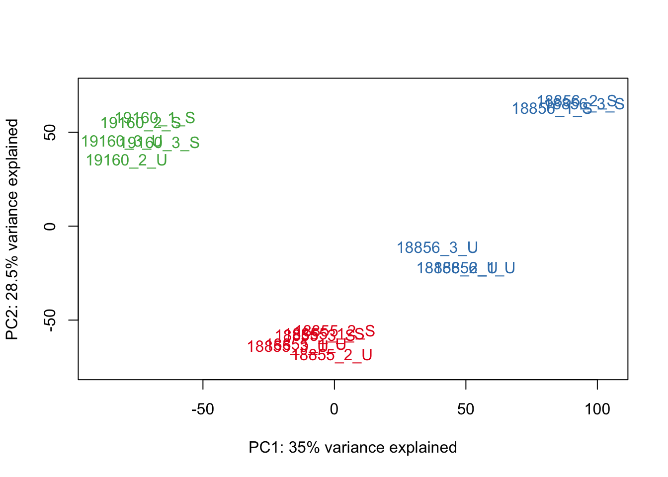
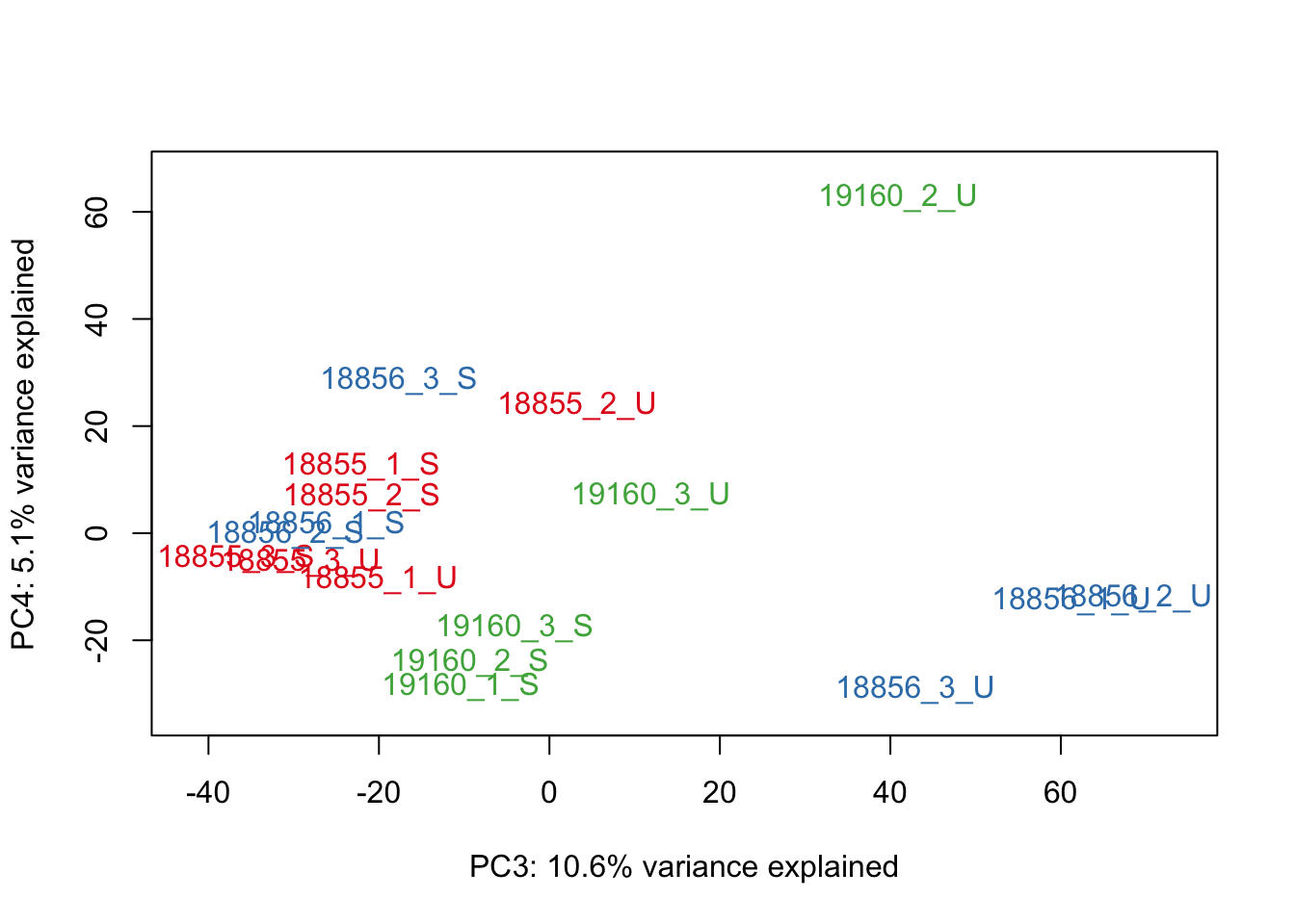
source("code/PCA_fn.R")PCA of normalized and filtered data
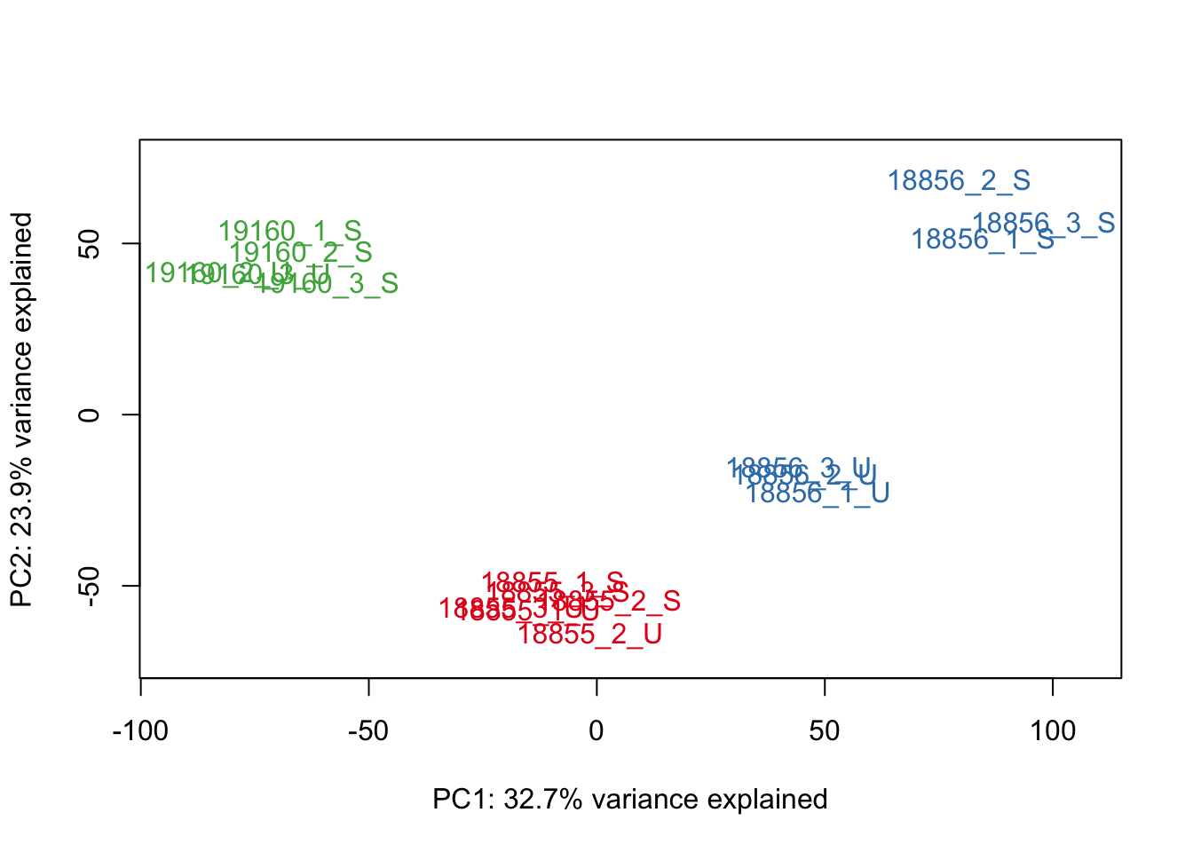
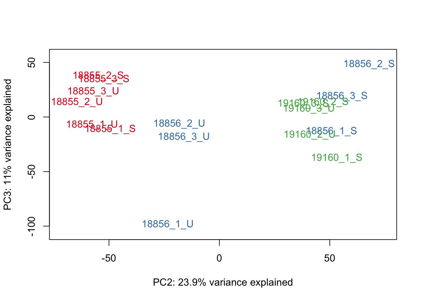
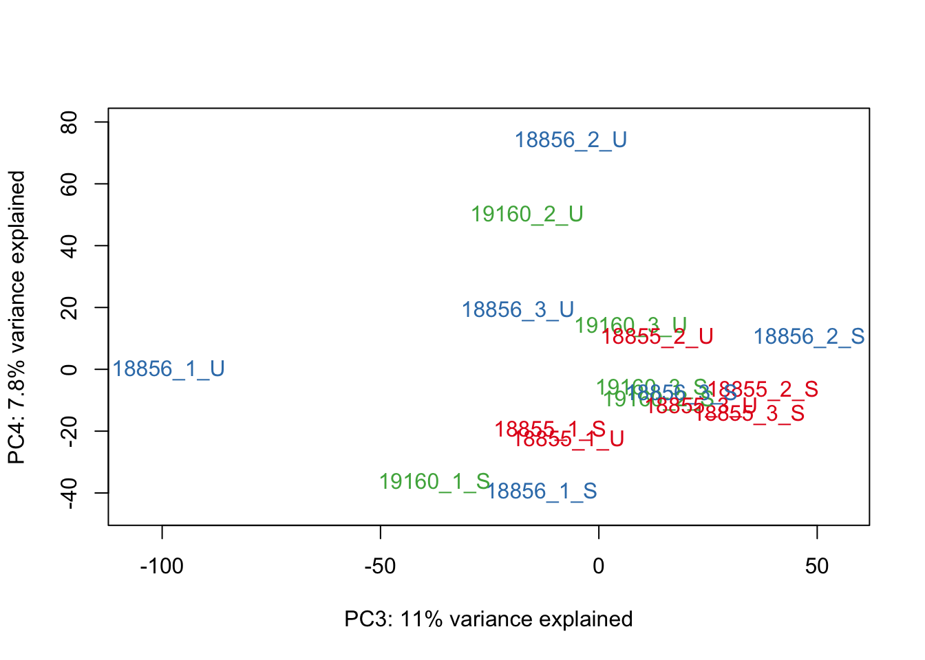
Here, we plot the samples represented by their sample IDs (more informative) and by symbols (for more asthetic presentation in figures).
# Perform PCA
pca_genes <- prcomp(t(filt_norm_counts), scale = T)
scores <- pca_genes$x

variances <- pca_genes$sdev^2
explained <- variances / sum(variances)
plot(pca_genes, main = "Variance per PC")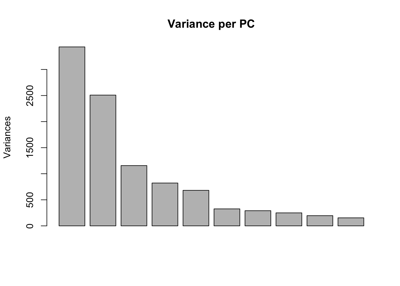
| Version | Author | Date |
|---|---|---|
| e3fbd0f | Anthony Hung | 2021-01-21 |
#Make PCA plots with the factors colored by Individual

### PCA norm+filt Data
for (n in 1:5){
  col.v <- pal[as.integer(sampleinfo$Individual)]
  plot_scores(pca_genes, scores, n, n+1, col.v)
}
| Version | Author | Date |
|---|---|---|
| e3fbd0f | Anthony Hung | 2021-01-21 |
| Version | Author | Date |
|---|---|---|
| e3fbd0f | Anthony Hung | 2021-01-21 |
| Version | Author | Date |
|---|---|---|
| e3fbd0f | Anthony Hung | 2021-01-21 |

| Version | Author | Date |
|---|---|---|
| e3fbd0f | Anthony Hung | 2021-01-21 |

| Version | Author | Date |
|---|---|---|
| e3fbd0f | Anthony Hung | 2021-01-21 |
#make PCA plots with symbols as treatment status and colors as individuals for figure
library(ggfortify)
autoplot(pca_genes, data = sampleinfo, colour = "Individual", shape = "treatment", size = 3) +
     theme_cowplot() +
     theme(legend.position = "none")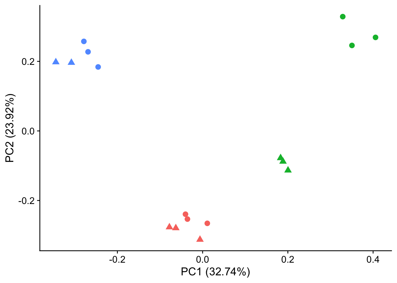
| Version | Author | Date |
|---|---|---|
| e3fbd0f | Anthony Hung | 2021-01-21 |
autoplot(pca_genes, data = sampleinfo, colour = "Individual", shape = "treatment") +
     theme_cowplot()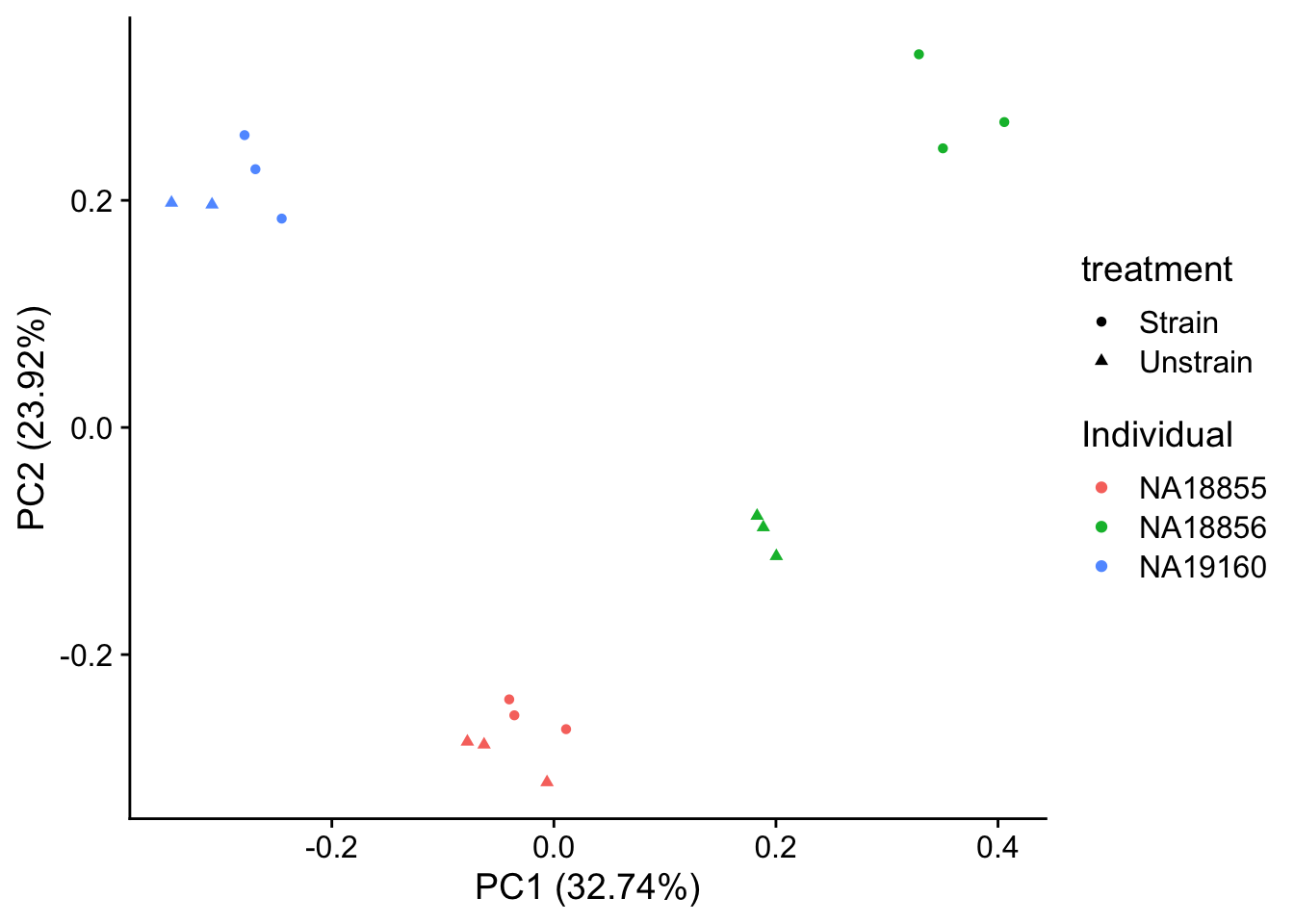
| Version | Author | Date |
|---|---|---|
| e3fbd0f | Anthony Hung | 2021-01-21 |
autoplot(pca_genes, data = sampleinfo, colour = "Individual", shape = "treatment", size = 3, x = 3, y = 4) +
     theme_cowplot() +
     theme(legend.position = "none")
| Version | Author | Date |
|---|---|---|
| e3fbd0f | Anthony Hung | 2021-01-21 |
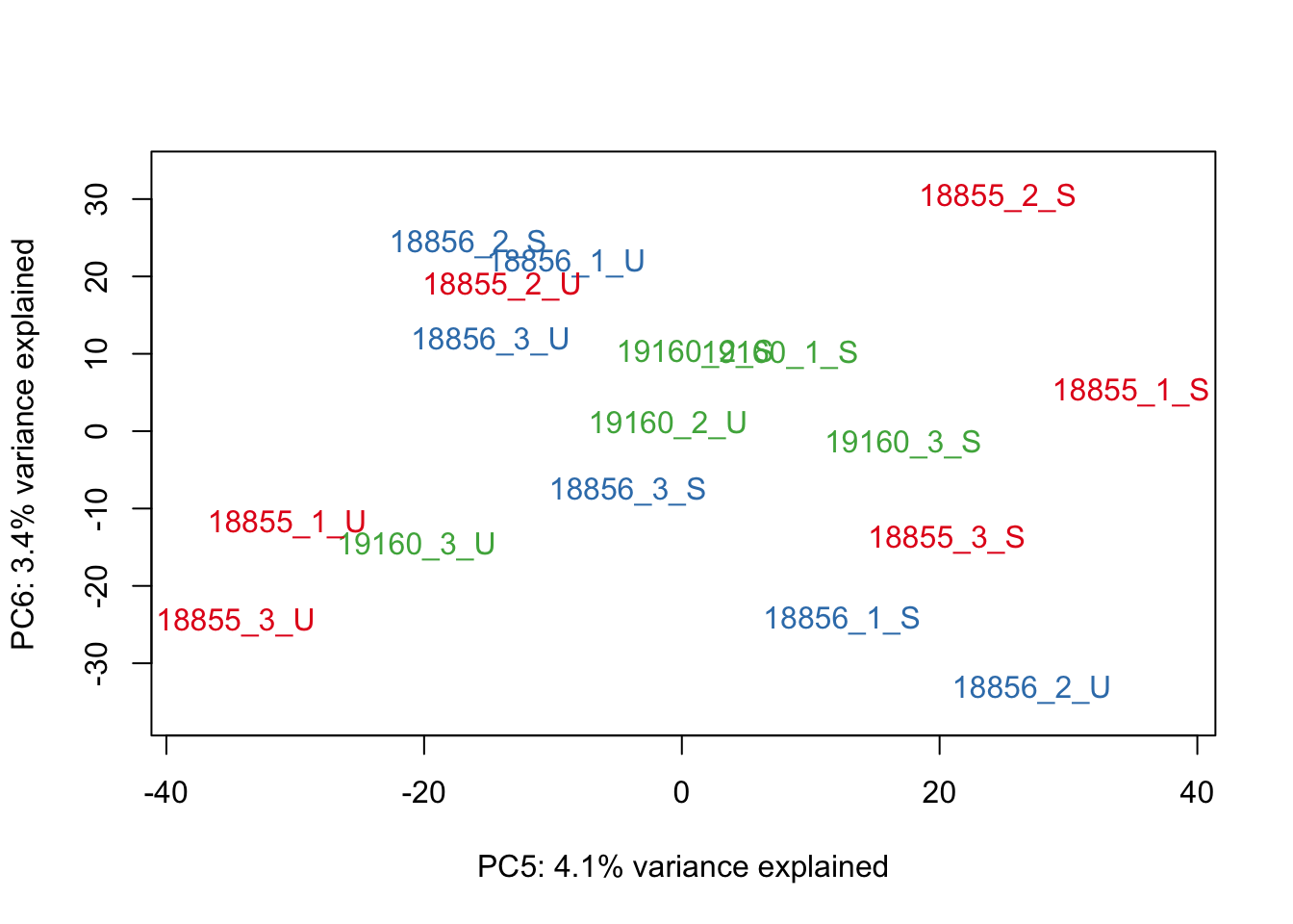
autoplot(pca_genes, data = sampleinfo, colour = "Individual", shape = "treatment", size = 3, x = 5, y = 6) +
     theme_cowplot() +
     theme(legend.position = "none")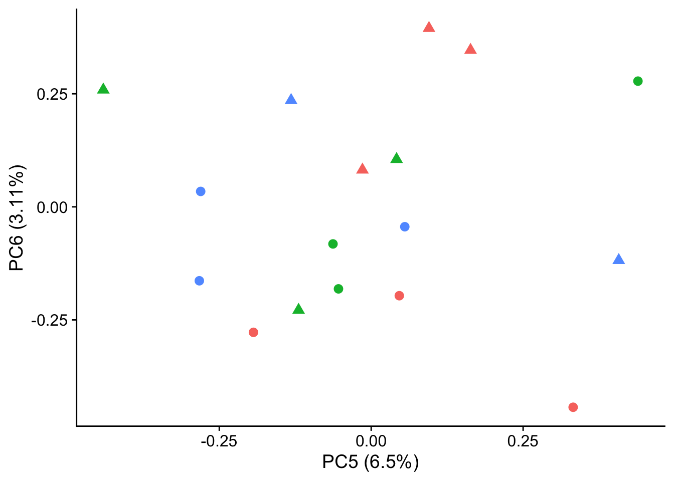
| Version | Author | Date |
|---|---|---|
| e3fbd0f | Anthony Hung | 2021-01-21 |
Examine correlations between top PCs and experimental variables
After performing our PCA, we calculate the correlation between the top 5 PCs and several recorded experimental variables, looking for significant correlations. We present them in a table as well as in a heatmap. We also find significant correlations after correction for multiple testing using a BH procedure.
# Calculate the relationship between each recorded covariate and the top 5 PCs.
p_comps <- 1:5
info <- sampleinfo %>%
     dplyr::select(c(Individual, Sex, Replicate, treatment, RIN, LibraryPrepBatch, LibSize)) #subset sample info for technical/biological variables

#Calculate correlations
pc_cov_cor <- matrix(nrow = ncol(info), ncol = length(p_comps),
                      dimnames = list(colnames(info), colnames(pca_genes$x)[p_comps]))

PC_pvalues <- matrix(data = NA, nrow = 5, ncol = 7, dimnames = list(c("PC1", "PC2", "PC3", "PC4", "PC5"), c("Individual", "Sex", "Replicate", "Treatment", "RIN", "LibraryPrepBatch", "LibSize")))

for (pc in p_comps) {
  for (covariate in 1:ncol(info)) {
        lm_result <- lm(pca_genes$x[, pc] ~ info[, covariate])
    r2 <- summary(lm_result)$r.squared
    fstat <- as.data.frame(summary(lm_result)$fstatistic)
    p_fstat <- 1-pf(fstat[1,], fstat[2,], fstat[3,])
    PC_pvalues[pc, covariate] <- p_fstat
    pc_cov_cor[covariate, pc] <- r2
  }
}
datatable(pc_cov_cor)
#BH adjust for multiple testing for the p-values for correlation
#Distribution of p-values adjusted by FDR
fdr_val <- p.adjust(PC_pvalues, method = "fdr", n = length(PC_pvalues))
fdr_val_order <- fdr_val[order(fdr_val)]
hist(fdr_val_order, ylab = "BH-adjusted p-values", main = "Distribution of Benjamini and Hochberg adjusted p-values", breaks = 10)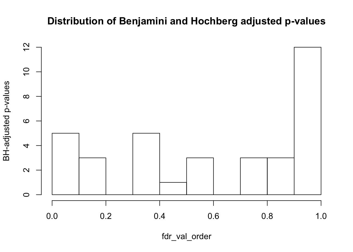
| Version | Author | Date |
|---|---|---|
| e3fbd0f | Anthony Hung | 2021-01-21 |
fdr_val <- matrix(fdr_val, nrow = 5, ncol = 7)
matrix_fdr_val <- matrix(fdr_val, nrow = 5, ncol = 7, dimnames = list(c("PC1", "PC2", "PC3", "PC4", "PC5"), c("Individual", "Sex", "Replicate", "Treatment", "RIN", "LibraryPrepBatch", "LibSize")))

#Get the coordinates of which variables/PC combinations are significant at FDR 5%

TorF_matrix_fdr <- matrix_fdr_val <=0.05
coor_to_check <- which(matrix_fdr_val <= 0.05, arr.ind=T)
coor_to_check <- as.data.frame(coor_to_check)
matrix_fdr_val
Individual Sex Replicate Treatment RIN LibraryPrepBatch
PC1 1.269735e-07 0.9336808625 0.9451743 0.9336809 0.07528095 0.9451743
PC2 4.590869e-04 0.0002579742 0.9451743 0.3946693 0.39466927 0.9622445
PC3 7.042737e-01 0.4631185780 0.1041397 0.3958344 0.94517429 0.5354247
PC4 8.288830e-01 0.5354246637 0.5354247 0.1041397 0.86144953 0.9451743
PC5 9.336809e-01 0.7042736812 0.3688630 0.9982813 0.94517429 0.3688630
LibSize
PC1 0.09539454
PC2 0.88477997
PC3 0.70427368
PC4 0.94517429
PC5 0.10413971coor_to_check # Individual has most significant correlation with pc1 and 2, and sex correlates with pc2 (probably due to the individual effect) row col
PC1 1 1
PC2 2 1
PC2.1 2 2#Convert to long format to plot in ggplot2
pc_cov_cor_2 <- as.data.frame(pc_cov_cor)
pc_cov_cor_2$variable <- rownames(pc_cov_cor)
pc_cov_cor_2 <- gather(pc_cov_cor_2, key = "pc", value = "cor", -variable)
head(pc_cov_cor_2) variable pc cor
1 Individual PC1 0.937736289
2 Sex PC1 0.012284763
3 Replicate PC1 0.005921329
4 treatment PC1 0.012967817
5 RIN PC1 0.378217485
6 LibraryPrepBatch PC1 0.001662314#Plot heatmap
d_heatmap <- pc_cov_cor_2
d_heatmap$variable <- factor(d_heatmap$variable,
levels = c("Individual", "Sex", "Replicate",
"treatment", "RIN", "LibraryPrepBatch", "LibSize"),
labels = c("Individual", "Sex", "Replicate",
"treatment", "RIN", "LibraryPrepBatch", "LibSize"))
pca_heat <- ggplot(d_heatmap, aes(x = pc, y = variable)) +
geom_tile(aes(fill = cor), colour = "white") +
scale_fill_gradient(low = "white", high = "red", limits = c(0, 1)) +
labs(x = "Principal Component", y = "",
title = "Correlation between principal components and experimental variables")
pca_heat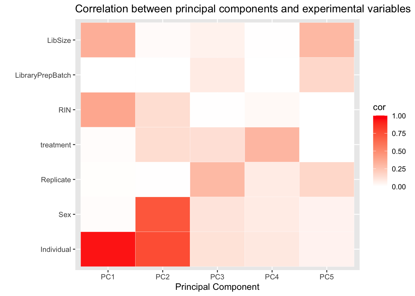
| Version | Author | Date |
|---|---|---|
| e3fbd0f | Anthony Hung | 2021-01-21 |
Remove unwanted variation using RUVSeq
After examining the correlation structure between major axes of variation and experimental variables in the unadjusted data, we are interested in modeling two factors of unwanted variation in the data. Here, we take advantage of the technical replicate structure of our study design and employ RUVs to fit these two unwanted sources of variation.
#Use RUVs (replicates)
replicates <- makeGroups(paste0(sampleinfo$Individual, sampleinfo$treatment))
x <- paste0(sampleinfo$Individual, sampleinfo$treatment)

#load data into expressionset
set <- newSeqExpressionSet(as.matrix(filt_counts$counts),
                           phenoData = data.frame(sampleinfo, row.names=colnames(filt_norm_counts)))
set
SeqExpressionSet (storageMode: lockedEnvironment)
assayData: 10486 features, 17 samples
element names: counts, normalizedCounts, offset
protocolData: none
phenoData
sampleNames: 18855_3_S 19160_3_S ... 18855_3_U (17 total)
varLabels: Sample_ID Individual ... LibSize (8 total)
varMetadata: labelDescription
featureData: none
experimentData: use 'experimentData(object)'
Annotation: #normalization
set <- betweenLaneNormalization(x = set, which = "upper", round = T)
#
set1 <- RUVs(x=set, cIdx = rownames(filt_counts), k=2, scIdx = replicates, round = F)
pData(set1) Sample_ID Individual Sex Replicate treatment RIN LibraryPrepBatch
18855_3_S 18855_3_S NA18855 F 3 Strain 10.0 2
19160_3_S 19160_3_S NA19160 M 3 Strain 10.0 2
18856_3_U 18856_3_U NA18856 M 3 Unstrain 10.0 2
18856_1_U 18856_1_U NA18856 M 1 Unstrain 9.9 1
18855_2_S 18855_2_S NA18855 F 2 Strain 10.0 1
18856_2_S 18856_2_S NA18856 M 2 Strain 9.6 1
19160_3_U 19160_3_U NA19160 M 3 Unstrain 10.0 2
18855_2_U 18855_2_U NA18855 F 2 Unstrain 10.0 1
19160_2_S 19160_2_S NA19160 M 2 Strain 10.0 1
18855_1_S 18855_1_S NA18855 F 1 Strain 9.9 1
18856_1_S 18856_1_S NA18856 M 1 Strain 8.5 1
19160_1_S 19160_1_S NA19160 M 1 Strain 9.9 1
19160_2_U 19160_2_U NA19160 M 2 Unstrain 10.0 1
18855_1_U 18855_1_U NA18855 F 1 Unstrain 10.0 1
18856_3_S 18856_3_S NA18856 M 3 Strain 9.6 2
18856_2_U 18856_2_U NA18856 M 2 Unstrain 9.5 1
18855_3_U 18855_3_U NA18855 F 3 Unstrain 10.0 2
LibSize W_1 W_2
18855_3_S 15419569 0.541963415 -1.1181740
19160_3_S 15177653 0.376349314 -1.4100700
18856_3_U 13722909 0.857248982 -0.8808562
18856_1_U 18647599 1.113674153 -1.5466409
18855_2_S 18256163 0.733375747 -0.7617020
18856_2_S 16782764 -0.051863231 -1.3484210
19160_3_U 19839604 0.224499121 -1.5560509
18855_2_U 18618691 0.665015743 -0.9464050
19160_2_S 16622407 0.308745015 -1.5149287
18855_1_S 19712744 0.626769726 -1.5366695
18856_1_S 13571439 1.038716806 -1.2664724
19160_1_S 20979958 0.461484490 -2.0300296
19160_2_U 20924281 0.002654243 -1.9184820
18855_1_U 20146697 0.649711618 -1.4110342
18856_3_S 15807863 0.728747075 -0.9909086
18856_2_U 15142152 0.359175096 -1.0809905
18855_3_U 18157918 0.487681866 -1.2290497Examine correlations between top PCs and experimental variables after RUVs
As above, we examine the correlations between top 5 PCs and experimental variables, but with the data adjusted for the two RUVs factors of unwanted variation.
# Perform PCA
pca_genes <- prcomp(t(set1@assayData$normalizedCounts), scale = T)
scores <- pca_genes$x

variances <- pca_genes$sdev^2
explained <- variances / sum(variances)
plot(pca_genes, main = "Variance per PC")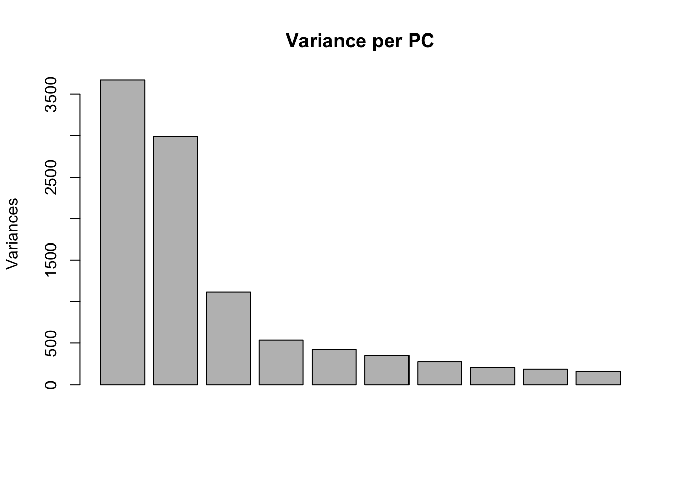
| Version | Author | Date |
|---|---|---|
| e3fbd0f | Anthony Hung | 2021-01-21 |
#Make PCA plots with the factors colored by Individual

### PCA norm+filt Data
for (n in 1:5){
  col.v <- pal[as.integer(sampleinfo$Individual)]
  plot_scores(pca_genes, scores, n, n+1, col.v)
}
| Version | Author | Date |
|---|---|---|
| e3fbd0f | Anthony Hung | 2021-01-21 |

| Version | Author | Date |
|---|---|---|
| e3fbd0f | Anthony Hung | 2021-01-21 |
| Version | Author | Date |
|---|---|---|
| e3fbd0f | Anthony Hung | 2021-01-21 |

| Version | Author | Date |
|---|---|---|
| e3fbd0f | Anthony Hung | 2021-01-21 |
| Version | Author | Date |
|---|---|---|
| e3fbd0f | Anthony Hung | 2021-01-21 |
#make PCA plots with symbols as treatment status and colors as individuals for figure
library(ggfortify)
autoplot(pca_genes, data = sampleinfo, colour = "Individual", shape = "treatment", size = 3) +
     theme_cowplot() +
     theme(legend.position = "none")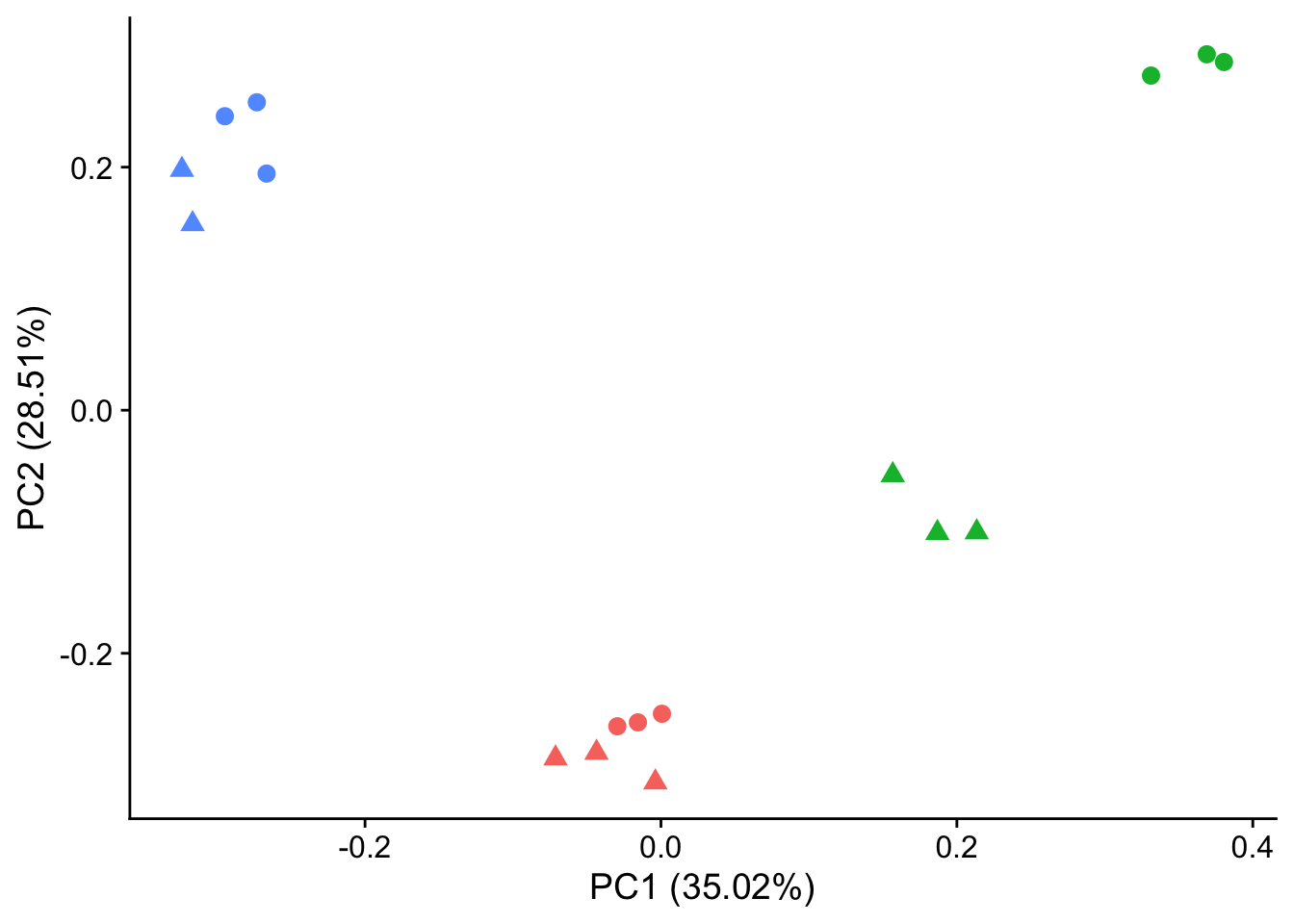
| Version | Author | Date |
|---|---|---|
| e3fbd0f | Anthony Hung | 2021-01-21 |
autoplot(pca_genes, data = sampleinfo, colour = "Individual", shape = "treatment") +
     theme_cowplot()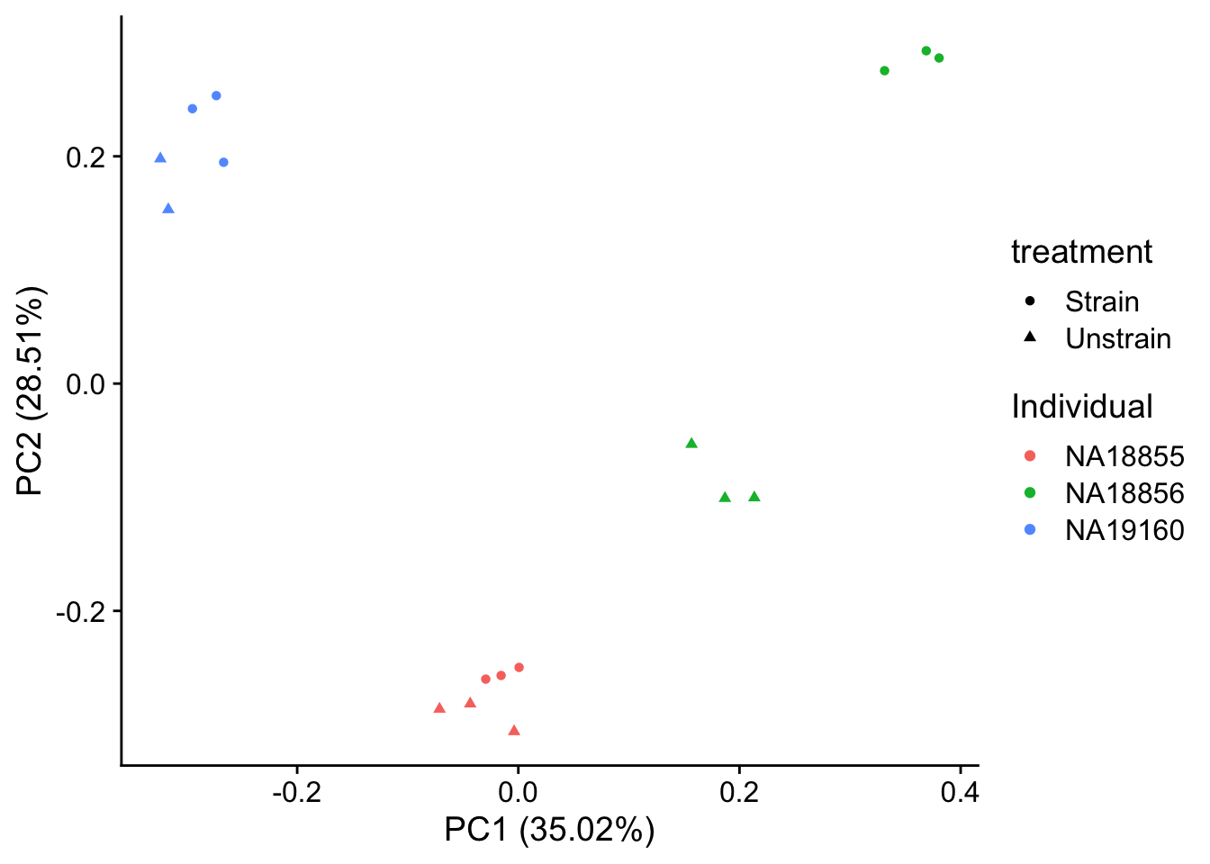
| Version | Author | Date |
|---|---|---|
| e3fbd0f | Anthony Hung | 2021-01-21 |
autoplot(pca_genes, data = sampleinfo, colour = "Individual", shape = "treatment", size = 3, x = 3, y = 4) +
     theme_cowplot() +
     theme(legend.position = "none")
| Version | Author | Date |
|---|---|---|
| e3fbd0f | Anthony Hung | 2021-01-21 |
autoplot(pca_genes, data = sampleinfo, colour = "Individual", shape = "treatment", size = 3, x = 5, y = 6) +
     theme_cowplot() +
     theme(legend.position = "none")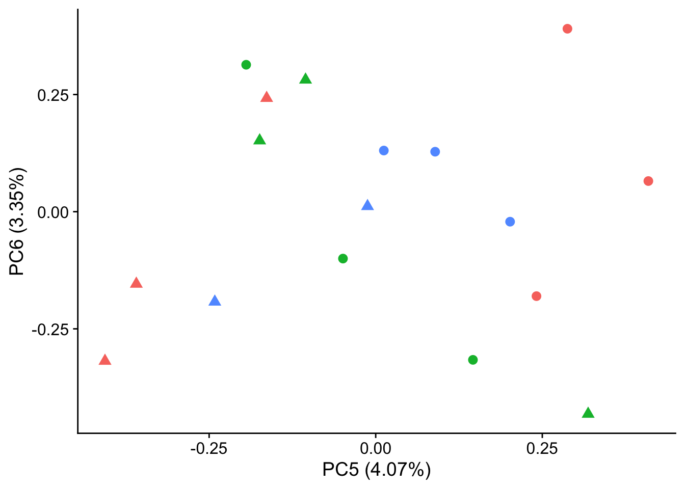
| Version | Author | Date |
|---|---|---|
| e3fbd0f | Anthony Hung | 2021-01-21 |
# Calculate the relationship between each recorded covariate and the top 5 PCs.
p_comps <- 1:5
info <- sampleinfo %>%
     dplyr::select(c(Individual, Sex, Replicate, treatment, RIN, LibraryPrepBatch, LibSize)) #subset sample info for technical/biological variables

#Calculate correlations
pc_cov_cor <- matrix(nrow = ncol(info), ncol = length(p_comps),
                      dimnames = list(colnames(info), colnames(pca_genes$x)[p_comps]))

PC_pvalues <- matrix(data = NA, nrow = 5, ncol = 7, dimnames = list(c("PC1", "PC2", "PC3", "PC4", "PC5"), c("Individual", "Sex", "Replicate", "Treatment", "RIN", "LibraryPrepBatch", "LibSize")))

for (pc in p_comps) {
  for (covariate in 1:ncol(info)) {
        lm_result <- lm(pca_genes$x[, pc] ~ info[, covariate])
    r2 <- summary(lm_result)$r.squared
    fstat <- as.data.frame(summary(lm_result)$fstatistic)
    p_fstat <- 1-pf(fstat[1,], fstat[2,], fstat[3,])
    PC_pvalues[pc, covariate] <- p_fstat
    pc_cov_cor[covariate, pc] <- r2
  }
}
datatable(pc_cov_cor)
#BH adjust for multiple testing for the p-values for correlation
#Distribution of p-values adjusted by FDR
fdr_val <- p.adjust(PC_pvalues, method = "fdr", n = length(PC_pvalues))
fdr_val_order <- fdr_val[order(fdr_val)]
hist(fdr_val_order, ylab = "BH-adjusted p-values", main = "Distribution of Benjamini and Hochberg adjusted p-values", breaks = 10)
| Version | Author | Date |
|---|---|---|
| e3fbd0f | Anthony Hung | 2021-01-21 |
fdr_val <- matrix(fdr_val, nrow = 5, ncol = 7)
matrix_fdr_val <- matrix(fdr_val, nrow = 5, ncol = 7, dimnames = list(c("PC1", "PC2", "PC3", "PC4", "PC5"), c("Individual", "Sex", "Replicate", "Treatment", "RIN", "LibraryPrepBatch", "LibSize")))

#Get the coordinates of which variables/PC combinations are significant at FDR 5%

TorF_matrix_fdr <- matrix_fdr_val <=0.05
coor_to_check <- which(matrix_fdr_val <= 0.05, arr.ind=T)
coor_to_check <- as.data.frame(coor_to_check)
matrix_fdr_val
Individual Sex Replicate Treatment RIN LibraryPrepBatch
PC1 8.046714e-08 0.9797494684 0.9797495 0.97974947 0.07413884 0.9797495
PC2 3.863803e-04 0.0001807959 0.9797495 0.42711188 0.42711188 0.9797495
PC3 4.283279e-01 0.2193110404 0.9797495 0.03943709 0.97974947 0.9797495
PC4 9.797495e-01 0.9797494684 0.9797495 0.97974947 0.97974947 0.9797495
PC5 9.921020e-01 0.9921020480 0.9797495 0.09477350 0.93296870 0.9329687
LibSize
PC1 0.1308890
PC2 0.9797495
PC3 0.9921020
PC4 0.5237645
PC5 0.9329687coor_to_check # Individual has most significant correlation with pc1 and 2, and sex correlates with pc2 (probably due to the individual effect) row col
PC1 1 1
PC2 2 1
PC2.1 2 2
PC3 3 4#Convert to long format to plot in ggplot2
pc_cov_cor_2 <- as.data.frame(pc_cov_cor)
pc_cov_cor_2$variable <- rownames(pc_cov_cor)
pc_cov_cor_2 <- gather(pc_cov_cor_2, key = "pc", value = "cor", -variable)
head(pc_cov_cor_2) variable pc cor
1 Individual PC1 0.941664115
2 Sex PC1 0.007266418
3 Replicate PC1 0.013020637
4 treatment PC1 0.010225547
5 RIN PC1 0.362169301
6 LibraryPrepBatch PC1 0.006470499#Plot heatmap
d_heatmap <- pc_cov_cor_2
d_heatmap$variable <- factor(d_heatmap$variable,
levels = c("Individual", "Sex", "Replicate",
"treatment", "RIN", "LibraryPrepBatch", "LibSize"),
labels = c("Individual", "Sex", "Replicate",
"treatment", "RIN", "LibraryPrepBatch", "LibSize"))
pca_heat <- ggplot(d_heatmap, aes(x = pc, y = variable)) +
geom_tile(aes(fill = cor), colour = "white") +
scale_fill_gradient(low = "white", high = "red", limits = c(0, 1)) +
labs(x = "Principal Component", y = "",
title = "Correlation between principal components and experimental variables")
pca_heat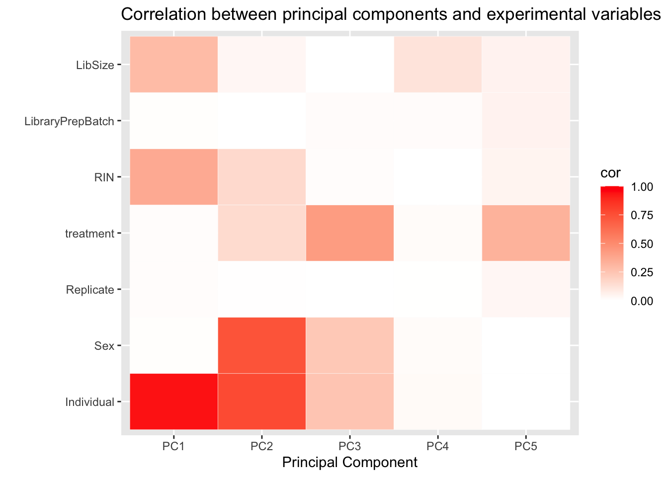
| Version | Author | Date |
|---|---|---|
| e3fbd0f | Anthony Hung | 2021-01-21 |
Save data and RUVs output for unwanted variation (contains the normalized/filtered count data as well as sample information data and W1+W2 values from RUVs)
saveRDS(set1, "data/RUVsOut.rds")
sessionInfo()R version 3.6.3 (2020-02-29)
Platform: x86_64-apple-darwin15.6.0 (64-bit)
Running under: macOS Catalina 10.15.7
Matrix products: default
BLAS: /Library/Frameworks/R.framework/Versions/3.6/Resources/lib/libRblas.0.dylib
LAPACK: /Library/Frameworks/R.framework/Versions/3.6/Resources/lib/libRlapack.dylib
locale:
[1] en_US.UTF-8/en_US.UTF-8/en_US.UTF-8/C/en_US.UTF-8/en_US.UTF-8
attached base packages:
[1] stats4 parallel stats graphics grDevices utils datasets
[8] methods base
other attached packages:
[1] ggfortify_0.4.10 dplyr_1.0.2
[3] RUVSeq_1.18.0 EDASeq_2.18.0
[5] ShortRead_1.42.0 GenomicAlignments_1.20.1
[7] SummarizedExperiment_1.14.1 DelayedArray_0.10.0
[9] matrixStats_0.56.0 Rsamtools_2.0.3
[11] GenomicRanges_1.36.1 GenomeInfoDb_1.20.0
[13] Biostrings_2.52.0 XVector_0.24.0
[15] IRanges_2.18.3 S4Vectors_0.22.1
[17] BiocParallel_1.18.1 Biobase_2.44.0
[19] BiocGenerics_0.30.0 tidyr_1.1.2
[21] DT_0.15 cowplot_1.1.1
[23] scales_1.1.1 RColorBrewer_1.1-2
[25] edgeR_3.26.8 limma_3.40.6
[27] reshape_0.8.8 ggplot2_3.3.2
[29] gplots_3.0.4
loaded via a namespace (and not attached):
[1] colorspace_1.4-1 hwriter_1.3.2 ellipsis_0.3.1
[4] rprojroot_1.3-2 fs_1.5.0 rstudioapi_0.11.0-9000
[7] farver_2.0.3 bit64_4.0.5 AnnotationDbi_1.46.1
[10] splines_3.6.3 R.methodsS3_1.8.1 DESeq_1.36.0
[13] geneplotter_1.62.0 knitr_1.29 jsonlite_1.7.0
[16] workflowr_1.6.2 annotate_1.62.0 png_0.1-7
[19] R.oo_1.24.0 compiler_3.6.3 httr_1.4.2
[22] backports_1.1.9 Matrix_1.2-18 later_1.1.0.1
[25] htmltools_0.5.0 prettyunits_1.1.1 tools_3.6.3
[28] gtable_0.3.0 glue_1.4.2 GenomeInfoDbData_1.2.1
[31] Rcpp_1.0.5 vctrs_0.3.4 gdata_2.18.0
[34] rtracklayer_1.44.4 crosstalk_1.1.0.1 xfun_0.16
[37] stringr_1.4.0 lifecycle_0.2.0 gtools_3.8.2
[40] XML_3.98-1.20 zlibbioc_1.30.0 MASS_7.3-52
[43] aroma.light_3.14.0 hms_0.5.3 promises_1.1.1
[46] yaml_2.2.1 gridExtra_2.3 memoise_1.1.0
[49] biomaRt_2.40.5 latticeExtra_0.6-29 stringi_1.4.6
[52] RSQLite_2.2.0 genefilter_1.66.0 GenomicFeatures_1.36.4
[55] caTools_1.18.0 rlang_0.4.7 pkgconfig_2.0.3
[58] bitops_1.0-6 evaluate_0.14 lattice_0.20-41
[61] purrr_0.3.4 labeling_0.3 htmlwidgets_1.5.1
[64] bit_4.0.4 tidyselect_1.1.0 plyr_1.8.6
[67] magrittr_1.5 R6_2.4.1 generics_0.0.2
[70] DBI_1.1.0 pillar_1.4.6 whisker_0.4
[73] withr_2.2.0 survival_3.2-3 RCurl_1.98-1.2
[76] tibble_3.0.3 crayon_1.3.4 KernSmooth_2.23-17
[79] rmarkdown_2.3 jpeg_0.1-8.1 progress_1.2.2
[82] locfit_1.5-9.4 grid_3.6.3 blob_1.2.1
[85] git2r_0.27.1 digest_0.6.25 xtable_1.8-4
[88] httpuv_1.5.4 R.utils_2.10.1 munsell_0.5.0