ggplot2

workflowr

• Summary
• Checks
• Past versions

Last updated: 2020-06-23

Checks: 7 0

Knit directory: MSTPsummerstatistics/

This reproducible R Markdown analysis was created with workflowr (version 1.5.0). The Checks tab describes the reproducibility checks that were applied when the results were created. The Past versions tab lists the development history.

---

R Markdown file: up-to-date

Great! Since the R Markdown file has been committed to the Git repository, you know the exact version of the code that produced these results.

Environment: empty

Great job! The global environment was empty. Objects defined in the global environment can affect the analysis in your R Markdown file in unknown ways. For reproduciblity it’s best to always run the code in an empty environment.

Seed: set.seed(20180927)

The command set.seed(20180927) was run prior to running the code in the R Markdown file. Setting a seed ensures that any results that rely on randomness, e.g. subsampling or permutations, are reproducible.

Session information: recorded

Great job! Recording the operating system, R version, and package versions is critical for reproducibility.

Cache: none

Nice! There were no cached chunks for this analysis, so you can be confident that you successfully produced the results during this run.

File paths: relative

Great job! Using relative paths to the files within your workflowr project makes it easier to run your code on other machines.

Repository version: ac9c26c

Great! You are using Git for version control. Tracking code development and connecting the code version to the results is critical for reproducibility. The version displayed above was the version of the Git repository at the time these results were generated.

Note that you need to be careful to ensure that all relevant files for the analysis have been committed to Git prior to generating the results (you can use wflow_publish or wflow_git_commit). workflowr only checks the R Markdown file, but you know if there are other scripts or data files that it depends on. Below is the status of the Git repository when the results were generated:

Ignored files:
    Ignored:    .DS_Store
    Ignored:    .RData
    Ignored:    .Rhistory
    Ignored:    .Rproj.user/
    Ignored:    analysis/.DS_Store
    Ignored:    analysis/.RData
    Ignored:    analysis/.Rhistory
    Ignored:    data/.DS_Store

Note that any generated files, e.g. HTML, png, CSS, etc., are not included in this status report because it is ok for generated content to have uncommitted changes.

---

These are the previous versions of the R Markdown and HTML files. If you’ve configured a remote Git repository (see ?wflow_git_remote), click on the hyperlinks in the table below to view them.

File	Version	Author	Date	Message
html	61e3892	Anthony Hung	2020-06-23	add cheatsheet links
html	2a37983	Anthony Hung	2020-06-23	Build site.
html	a1a0bd4	Anthony Hung	2020-06-23	Build site.
html	cdeb6c5	Anthony Hung	2020-06-22	Build site.
html	14c0094	Anthony Hung	2020-06-12	Build site.
html	1378fca	Anthony Hung	2020-06-12	Build site.
html	9bb0ed6	Anthony Hung	2020-05-12	Build site.
html	2114e6c	Anthony Hung	2020-05-10	Build site.
html	29c91df	Anthony Hung	2020-05-10	Build site.
html	a6d0787	Anthony Hung	2020-05-09	Build site.
html	e18c369	Anthony Hung	2020-05-02	Build site.
html	0e6b6d0	Anthony Hung	2020-04-30	Build site.
html	5cbe42c	Anthony Hung	2020-04-23	Build site.
html	4e08935	Anthony Hung	2020-03-30	Build site.
Rmd	058310e	Anthony Hung	2020-03-30	resampling lesson
html	310d040	Anthony Hung	2020-02-20	Build site.
Rmd	e02f5ce	Anthony Hung	2020-02-20	add dataviz
html	e02f5ce	Anthony Hung	2020-02-20	add dataviz

---

Data visualization in many dimensions with ggplot2

Load data and libraries

library(ggplot2)
cars <- mtcars
?mtcars

Examine structure of data

These data contain 32 observations on cars across 11 different variables. Some of these variables (e.g. mpg) are numeric, while others (e.g. cyl) are factors. Notice that these data are in “tidy” format, meaning that:

1. Each variable forms a column.

2. Each observation forms a row.

3. Each type of observational unit forms a table.

dim(cars)

[1] 32 11

head(cars)

                   mpg cyl disp  hp drat    wt  qsec vs am gear carb
Mazda RX4         21.0   6  160 110 3.90 2.620 16.46  0  1    4    4
Mazda RX4 Wag     21.0   6  160 110 3.90 2.875 17.02  0  1    4    4
Datsun 710        22.8   4  108  93 3.85 2.320 18.61  1  1    4    1
Hornet 4 Drive    21.4   6  258 110 3.08 3.215 19.44  1  0    3    1
Hornet Sportabout 18.7   8  360 175 3.15 3.440 17.02  0  0    3    2
Valiant           18.1   6  225 105 2.76 3.460 20.22  1  0    3    1

Plot showing 2 dimensions

Let’s examine the relationship between two variables, mpg and wt:

ggplot(data = cars) + #data layer
  geom_point(aes(x = wt, y = mpg)) #geom layer, aesthetics layer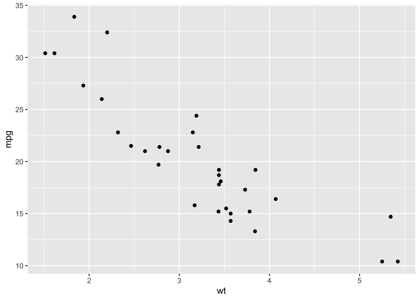

Past versions of unnamed-chunk-3-1.png

Version	Author	Date
61e3892	Anthony Hung	2020-06-23
5cbe42c	Anthony Hung	2020-04-23
e02f5ce	Anthony Hung	2020-02-20

Plot showing 3 dimensions

Now let’s color by cylinder number. What is important to take into account for the cylinder variable?

ggplot(data = cars) + #data layer
  geom_point(aes(x = wt, y = mpg, color = cyl)) #geom layer, aesthetics layer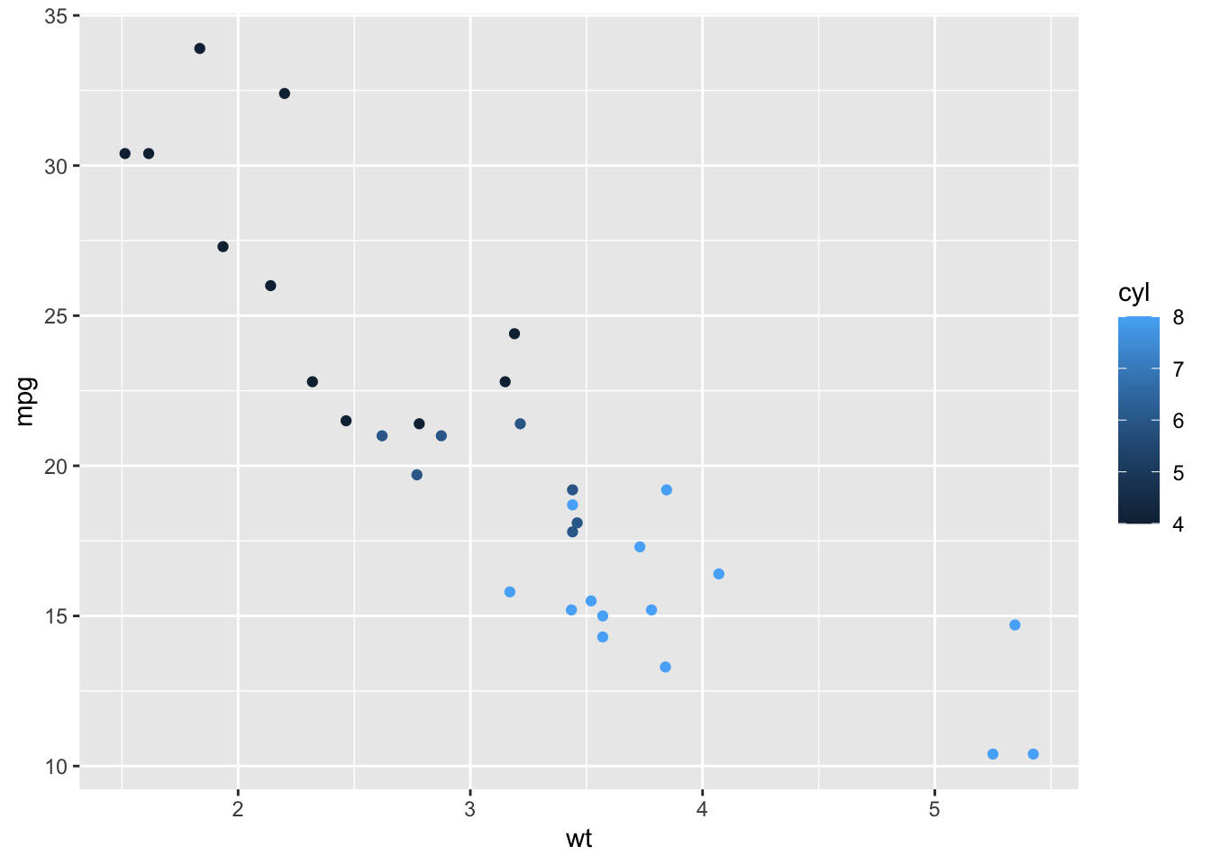

Past versions of unnamed-chunk-4-1.png

Version	Author	Date
61e3892	Anthony Hung	2020-06-23
5cbe42c	Anthony Hung	2020-04-23
e02f5ce	Anthony Hung	2020-02-20

ggplot(data = cars) + #data layer
  geom_point(aes(x = wt, y = mpg, size = factor(cyl))) #geom layer, aesthetics layer, color

Warning: Using size for a discrete variable is not advised.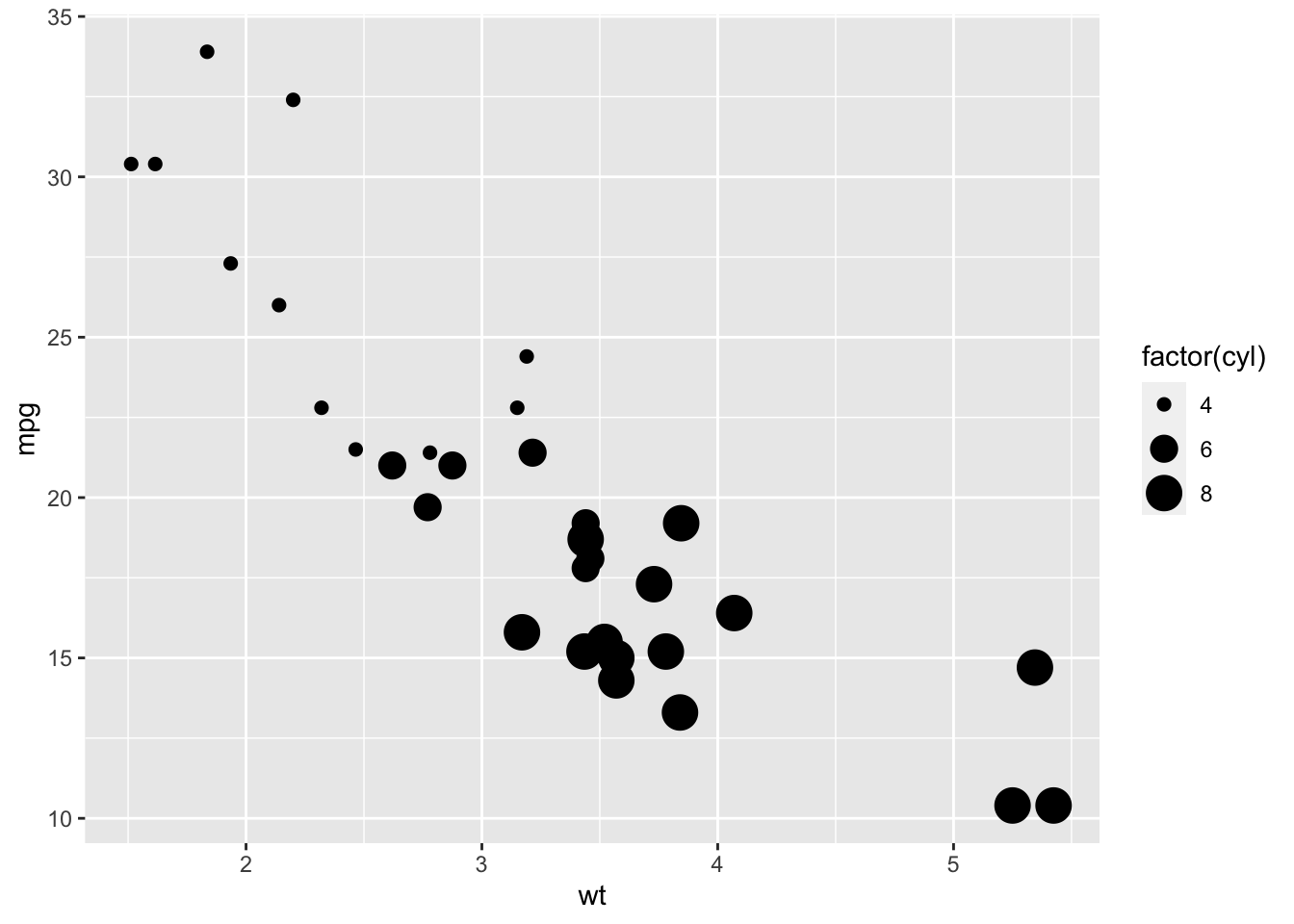

Past versions of unnamed-chunk-4-2.png

Version	Author	Date
61e3892	Anthony Hung	2020-06-23
5cbe42c	Anthony Hung	2020-04-23
e02f5ce	Anthony Hung	2020-02-20

ggplot(data = cars) + #data layer
  geom_point(aes(x = wt, y = mpg, shape = factor(cyl))) #geom layer, aesthetics layer, color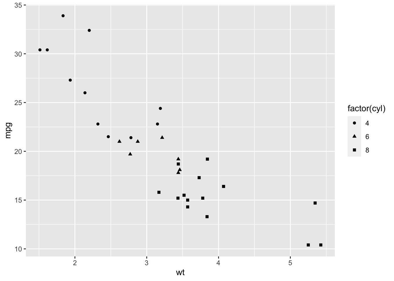

Past versions of unnamed-chunk-4-3.png

Version	Author	Date
61e3892	Anthony Hung	2020-06-23
5cbe42c	Anthony Hung	2020-04-23
e02f5ce	Anthony Hung	2020-02-20

ggplot(data = cars) + #data layer
  geom_point(aes(x = wt, y = mpg, color = factor(cyl))) #geom layer, aesthetics layer, color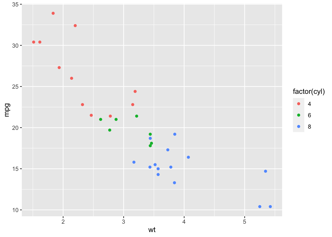

Past versions of unnamed-chunk-4-4.png

Version	Author	Date
61e3892	Anthony Hung	2020-06-23
5cbe42c	Anthony Hung	2020-04-23
e02f5ce	Anthony Hung	2020-02-20

Plot showing 4 dimensions

What if we’re interested in the same plot as above, but separated by automatic vs manual transmissions?

ggplot(data = cars) + #data layer
  geom_point(aes(x = wt, y = mpg, color = factor(cyl))) + #geom layer, aesthetics layer, color
  facet_wrap(~factor(am)) #facet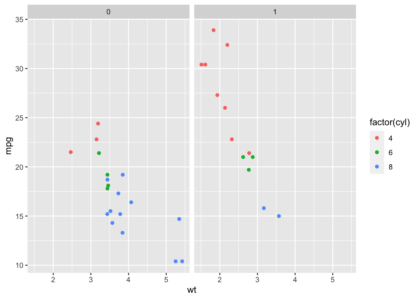

Past versions of unnamed-chunk-5-1.png

Version	Author	Date
61e3892	Anthony Hung	2020-06-23
5cbe42c	Anthony Hung	2020-04-23
e02f5ce	Anthony Hung	2020-02-20

#rename factor labels
cars$am <- as.factor(cars$am)
levels(cars$am) <- c("automatic", "manual")

ggplot(data = cars) + #data layer
  geom_point(aes(x = wt, y = mpg, color = factor(cyl))) + #geom layer, aesthetics layer, color
  facet_wrap(~am) #facet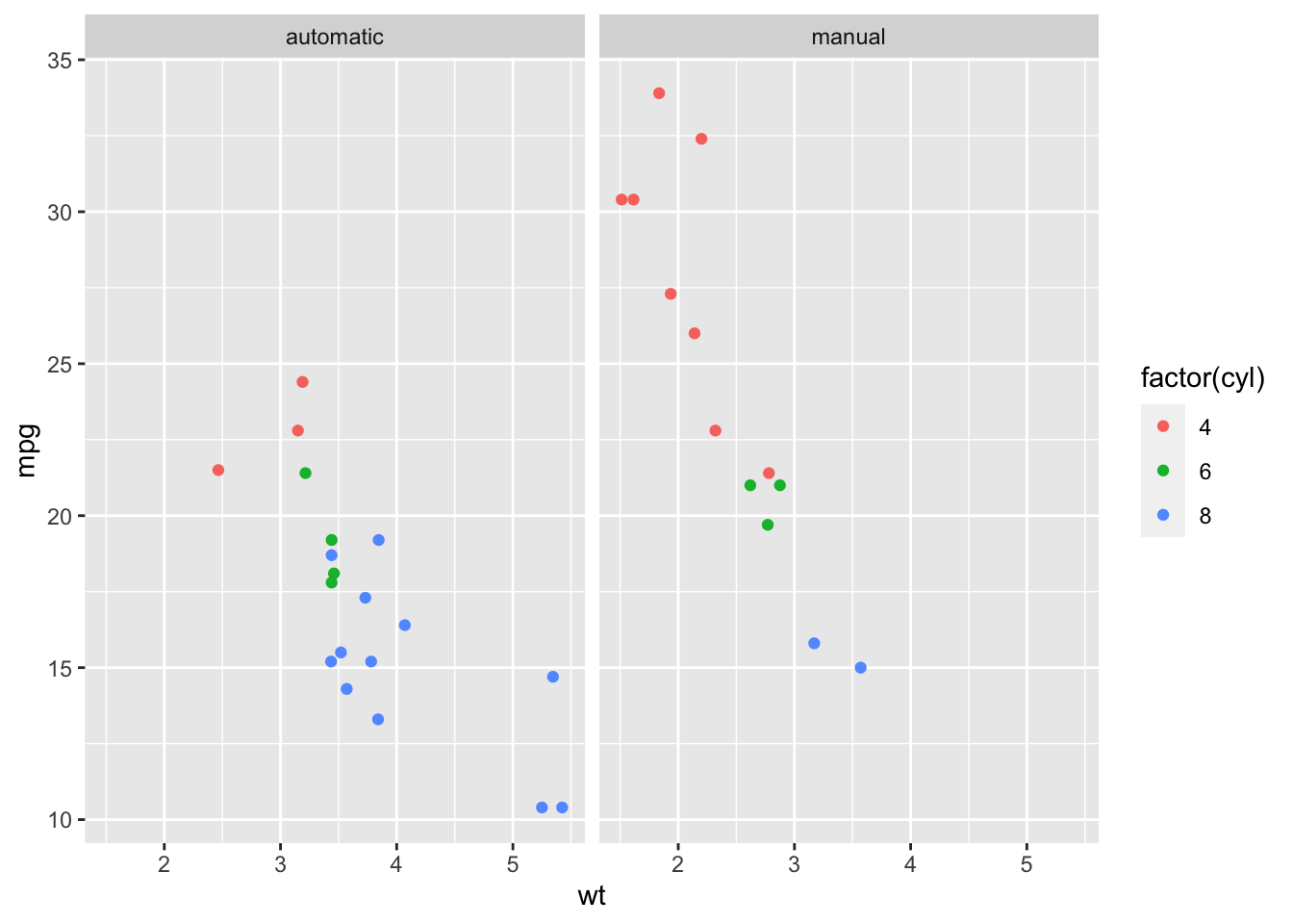

Past versions of unnamed-chunk-5-2.png

Version	Author	Date
61e3892	Anthony Hung	2020-06-23
5cbe42c	Anthony Hung	2020-04-23
e02f5ce	Anthony Hung	2020-02-20

Plot showing 5 dimensions

cars$vs <- as.factor(cars$vs)
levels(cars$vs) <- c("V-shaped engine", "straight engine")

ggplot(data = cars) + #data layer
  geom_point(aes(x = wt, y = mpg, color = factor(cyl))) + #geom layer, aesthetics layer, color
  facet_grid(vs~am) #facet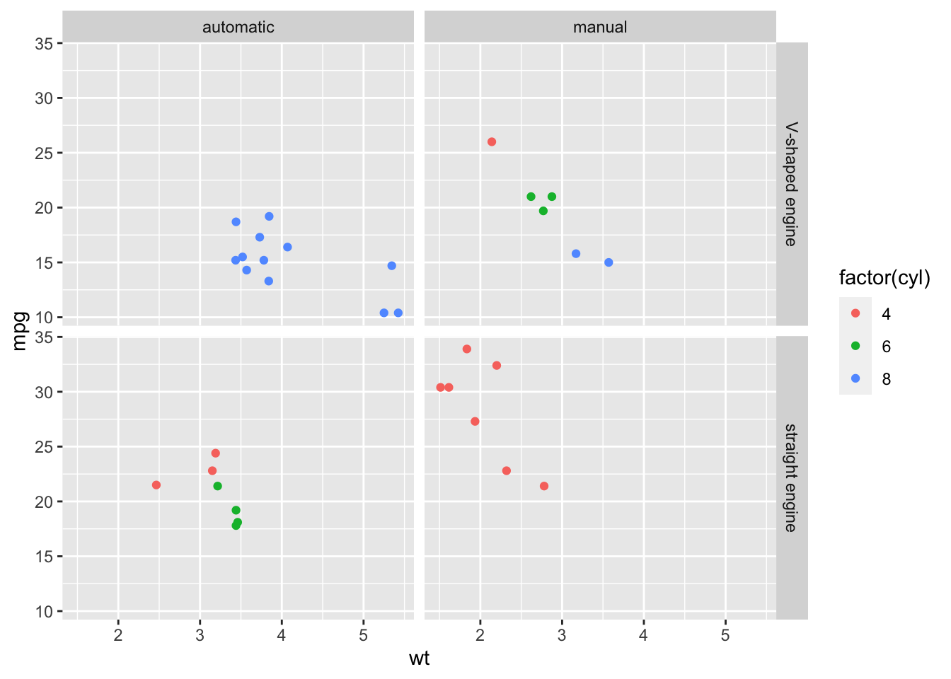

Past versions of unnamed-chunk-6-1.png

Version	Author	Date
61e3892	Anthony Hung	2020-06-23
5cbe42c	Anthony Hung	2020-04-23
e02f5ce	Anthony Hung	2020-02-20

Gone too far?

ggplot(data = cars) + #data layer
  geom_point(aes(x = wt, y = mpg, color = factor(cyl), size = disp, shape = factor(gear))) + #geom layer, aesthetics layer, color
  facet_grid(vs~am)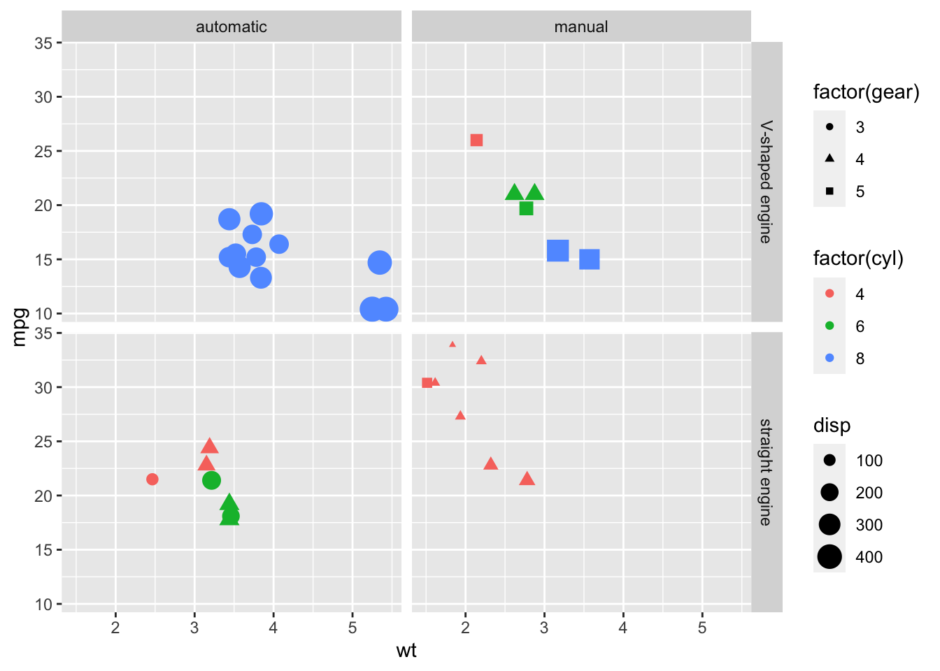

Past versions of unnamed-chunk-7-1.png

Version	Author	Date
61e3892	Anthony Hung	2020-06-23
5cbe42c	Anthony Hung	2020-04-23
e02f5ce	Anthony Hung	2020-02-20

Additional points

Adding labels

labeled_plot <- ggplot(data = cars) + #data layer
  geom_point(aes(x = wt, y = mpg, color = factor(cyl))) + #geom layer, aesthetics layer, color
  ggtitle("Relationship between mpg and weight \n in mtcars") + 
  xlab("weight (1000 lbs)") + 
  ylab("miles per gallon (mpg)") +
  labs(color = "Cylinder type")

labeled_plot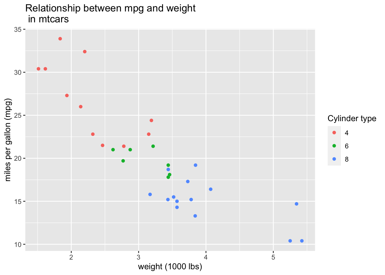

Past versions of unnamed-chunk-8-1.png

Version	Author	Date
61e3892	Anthony Hung	2020-06-23
5cbe42c	Anthony Hung	2020-04-23
e02f5ce	Anthony Hung	2020-02-20

Choosing colors

cylinder_colors <- c("#035AA6", "#F2AE2E", "#F23D3D")

labeled_plot +
  scale_color_manual(values=cylinder_colors)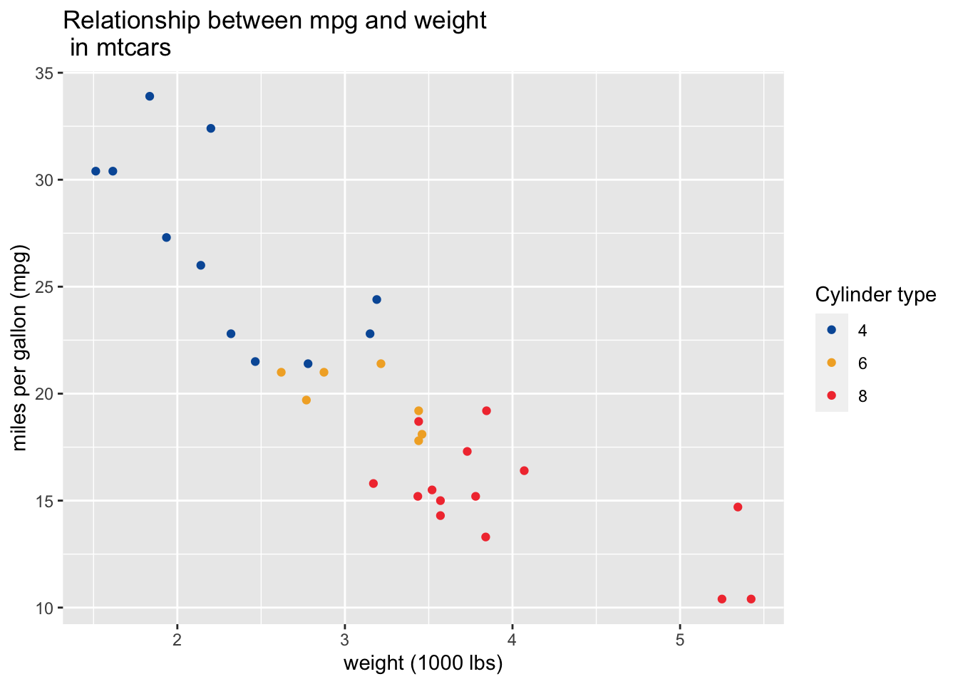

Past versions of unnamed-chunk-9-1.png

Version	Author	Date
61e3892	Anthony Hung	2020-06-23
5cbe42c	Anthony Hung	2020-04-23
e02f5ce	Anthony Hung	2020-02-20

Reordering factors

cars$cyl <- factor(cars$cyl)
cars$cyl <- factor(cars$cyl, levels(cars$cyl)[c(3,2,1)])

ggplot(data = cars) + #data layer
  geom_point(aes(x = wt, y = mpg, color = cyl)) + #geom layer, aesthetics layer, color
  ggtitle("Relationship between mpg and weight \n in mtcars") + 
  xlab("weight (1000 lbs)") + 
  ylab("miles per gallon (mpg)") +
  labs(color = "Cylinder type") +
  scale_color_manual(values=cylinder_colors)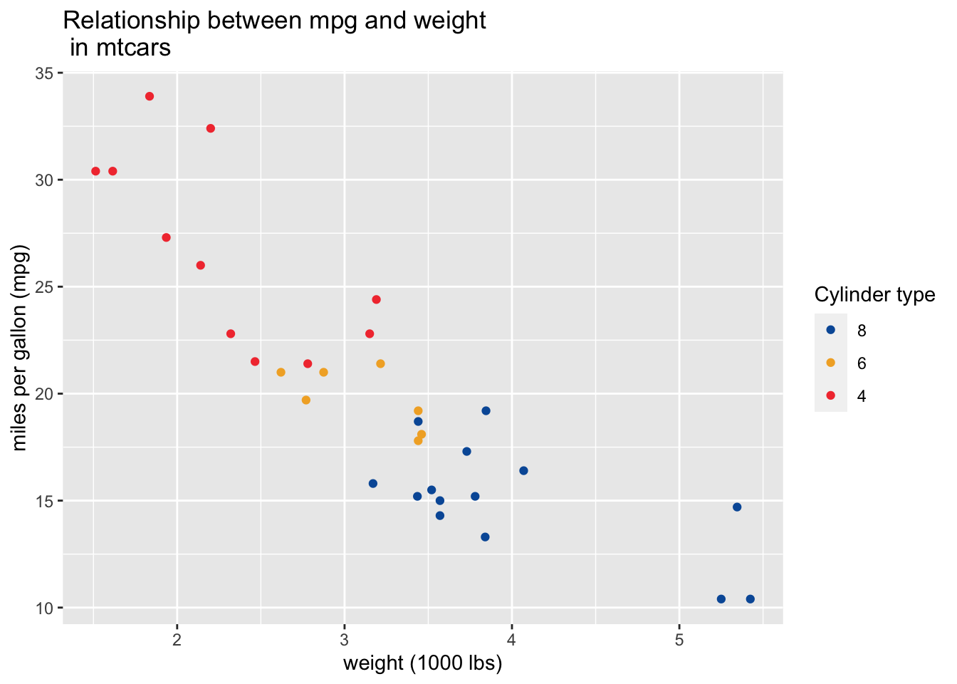

Past versions of unnamed-chunk-10-1.png

Version	Author	Date
61e3892	Anthony Hung	2020-06-23
5cbe42c	Anthony Hung	2020-04-23
e02f5ce	Anthony Hung	2020-02-20

Adding statistics

Remember, we are working with the grammar of graphics so we can add as many geoms as we want/need to our plot!

labeled_plot + 
  geom_smooth(aes(x = wt, y = mpg, color = factor(cyl)), method = "lm", se = FALSE) #additional geoms inherit data and aesthetics from the predefined plot

`geom_smooth()` using formula 'y ~ x'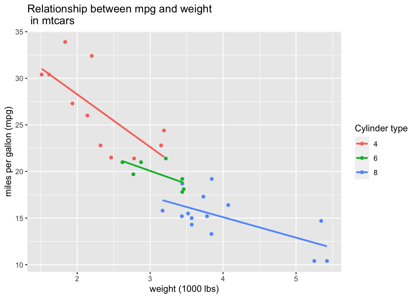

Past versions of unnamed-chunk-11-1.png

Version	Author	Date
61e3892	Anthony Hung	2020-06-23
5cbe42c	Anthony Hung	2020-04-23
e02f5ce	Anthony Hung	2020-02-20

#we can also define a new dataset for an additional geom
library(dplyr)

Attaching package: 'dplyr'

The following objects are masked from 'package:stats':

    filter, lag

The following objects are masked from 'package:base':

    intersect, setdiff, setequal, union

means <- cars %>% 
  group_by(cyl) %>% 
  summarise(mean.wt = mean(wt), mean.mpg = mean(mpg))
means

# A tibble: 3 x 3
  cyl   mean.wt mean.mpg
  <fct>   <dbl>    <dbl>
1 8        4.00     15.1
2 6        3.12     19.7
3 4        2.29     26.7

labeled_plot + 
  geom_point(data = means, aes(x = mean.wt, y = mean.mpg, color = cyl), size = 10, alpha = 0.5) +
  scale_color_manual(values=c(cylinder_colors))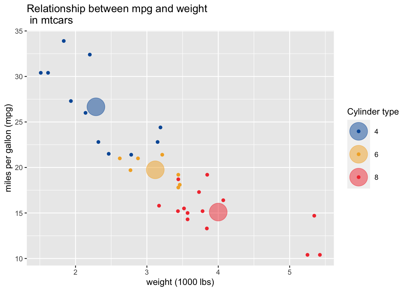

Past versions of unnamed-chunk-11-2.png

Version	Author	Date
61e3892	Anthony Hung	2020-06-23
5cbe42c	Anthony Hung	2020-04-23
e02f5ce	Anthony Hung	2020-02-20

Themes

library(ggthemes)
labeled_plot + 
  theme_fivethirtyeight()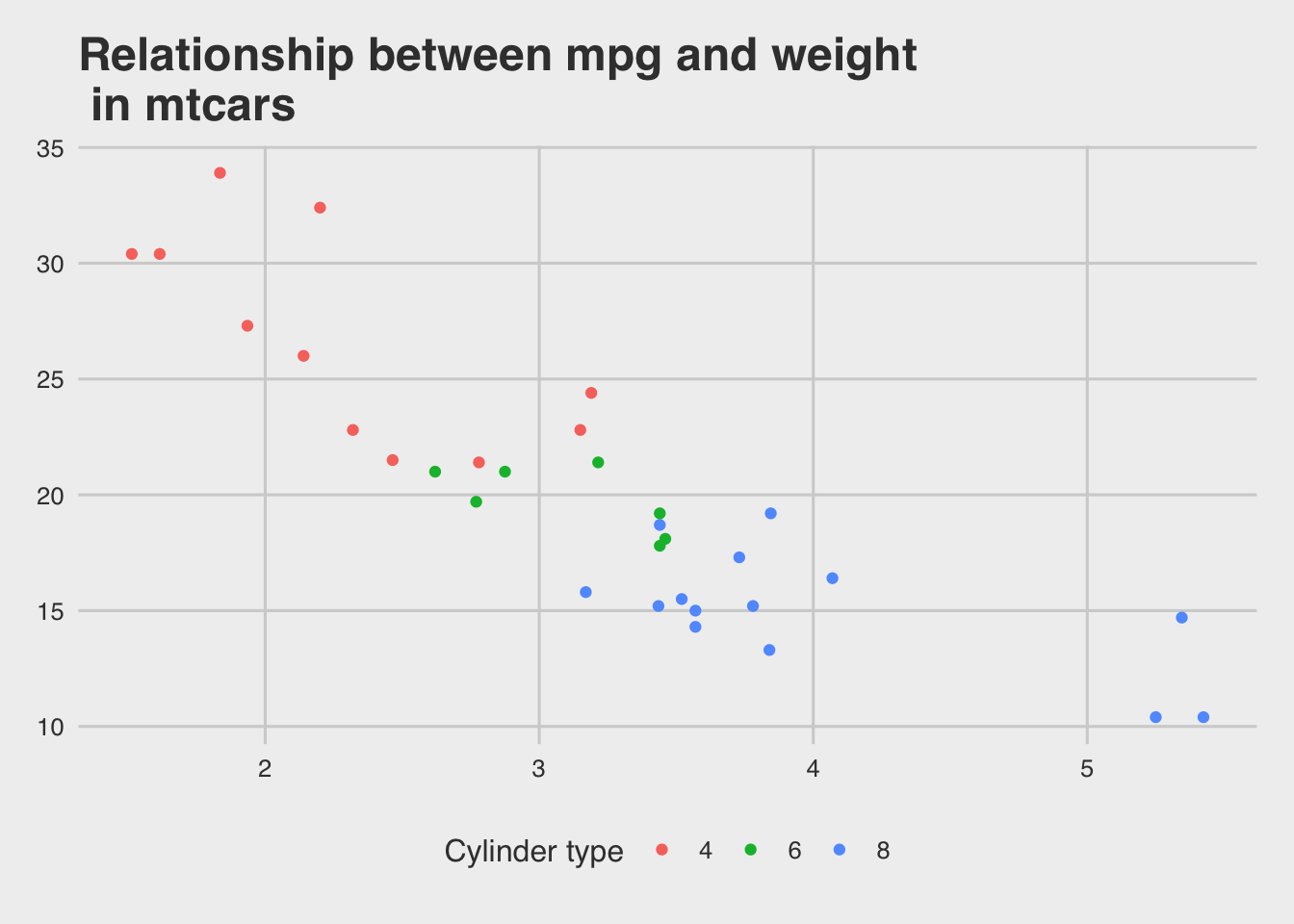

Past versions of unnamed-chunk-12-1.png

Version	Author	Date
61e3892	Anthony Hung	2020-06-23
5cbe42c	Anthony Hung	2020-04-23
e02f5ce	Anthony Hung	2020-02-20

Exercises

avocado_data <- read.csv('data/avocado.csv')
head(avocado_data)

  X       Date AveragePrice Total.Volume   X4046     X4225  X4770 Total.Bags
1 0 2015-12-27         1.33     64236.62 1036.74  54454.85  48.16    8696.87
2 1 2015-12-20         1.35     54876.98  674.28  44638.81  58.33    9505.56
3 2 2015-12-13         0.93    118220.22  794.70 109149.67 130.50    8145.35
4 3 2015-12-06         1.08     78992.15 1132.00  71976.41  72.58    5811.16
5 4 2015-11-29         1.28     51039.60  941.48  43838.39  75.78    6183.95
6 5 2015-11-22         1.26     55979.78 1184.27  48067.99  43.61    6683.91
  Small.Bags Large.Bags XLarge.Bags         type year region
1    8603.62      93.25           0 conventional 2015 Albany
2    9408.07      97.49           0 conventional 2015 Albany
3    8042.21     103.14           0 conventional 2015 Albany
4    5677.40     133.76           0 conventional 2015 Albany
5    5986.26     197.69           0 conventional 2015 Albany
6    6556.47     127.44           0 conventional 2015 Albany

dim(avocado_data)

[1] 18249    14

The above code chunk loads the avocado dataset, which contains data on avocado prices in different US regions between 2015-2018. Desriptions of what each of the columns mean can be found here: https://www.kaggle.com/neuromusic/avocado-prices.

1. Pick and create out a visualization that compares the number of Total bags, small bags, large bags, and extra large bags sold each year in each region.

2. Your choice! Pick any number of columns/entries you are interested in and create a visualization that says something interesting about the data.

Session information

sessionInfo()

R version 3.6.3 (2020-02-29)
Platform: x86_64-apple-darwin15.6.0 (64-bit)
Running under: macOS Catalina 10.15.5

Matrix products: default
BLAS:   /Library/Frameworks/R.framework/Versions/3.6/Resources/lib/libRblas.0.dylib
LAPACK: /Library/Frameworks/R.framework/Versions/3.6/Resources/lib/libRlapack.dylib

locale:
[1] en_US.UTF-8/en_US.UTF-8/en_US.UTF-8/C/en_US.UTF-8/en_US.UTF-8

attached base packages:
[1] stats     graphics  grDevices utils     datasets  methods   base     

other attached packages:
[1] ggthemes_4.2.0 dplyr_0.8.5    ggplot2_3.3.0 

loaded via a namespace (and not attached):
 [1] Rcpp_1.0.4.6     compiler_3.6.3   pillar_1.4.3     later_1.0.0     
 [5] git2r_0.26.1     workflowr_1.5.0  tools_3.6.3      digest_0.6.25   
 [9] lattice_0.20-38  nlme_3.1-144     evaluate_0.14    lifecycle_0.2.0 
[13] tibble_3.0.1     gtable_0.3.0     mgcv_1.8-31      pkgconfig_2.0.3 
[17] rlang_0.4.5      Matrix_1.2-18    cli_2.0.2        yaml_2.2.1      
[21] xfun_0.12        withr_2.1.2      stringr_1.4.0    knitr_1.26      
[25] fs_1.3.1         vctrs_0.2.4      rprojroot_1.3-2  grid_3.6.3      
[29] tidyselect_1.0.0 glue_1.4.0       R6_2.4.1         fansi_0.4.1     
[33] rmarkdown_1.18   farver_2.0.3     purrr_0.3.4      magrittr_1.5    
[37] whisker_0.4      splines_3.6.3    backports_1.1.6  scales_1.1.0    
[41] promises_1.1.0   htmltools_0.4.0  ellipsis_0.3.0   assertthat_0.2.1
[45] colorspace_1.4-1 httpuv_1.5.2     labeling_0.3     utf8_1.1.4      
[49] stringi_1.4.5    munsell_0.5.0    crayon_1.3.4