Last updated: 2020-06-23

Checks: 7 0

Knit directory: MSTPsummerstatistics/

This reproducible R Markdown analysis was created with workflowr (version 1.5.0). The Checks tab describes the reproducibility checks that were applied when the results were created. The Past versions tab lists the development history.

R Markdown file: up-to-date

Great! Since the R Markdown file has been committed to the Git repository, you know the exact version of the code that produced these results.

Environment: empty

Great job! The global environment was empty. Objects defined in the global environment can affect the analysis in your R Markdown file in unknown ways. For reproduciblity it’s best to always run the code in an empty environment.

Seed: set.seed(20180927)

The command set.seed(20180927) was run prior to running the code in the R Markdown file. Setting a seed ensures that any results that rely on randomness, e.g. subsampling or permutations, are reproducible.

Session information: recorded

Great job! Recording the operating system, R version, and package versions is critical for reproducibility.

Cache: none

Nice! There were no cached chunks for this analysis, so you can be confident that you successfully produced the results during this run.

File paths: relative

Great job! Using relative paths to the files within your workflowr project makes it easier to run your code on other machines.

Repository version: ac9c26c

Great! You are using Git for version control. Tracking code development and connecting the code version to the results is critical for reproducibility. The version displayed above was the version of the Git repository at the time these results were generated.

Note that you need to be careful to ensure that all relevant files for the analysis have been committed to Git prior to generating the results (you can use wflow_publish or wflow_git_commit). workflowr only checks the R Markdown file, but you know if there are other scripts or data files that it depends on. Below is the status of the Git repository when the results were generated:


Ignored files:
    Ignored:    .DS_Store
    Ignored:    .RData
    Ignored:    .Rhistory
    Ignored:    .Rproj.user/
    Ignored:    analysis/.DS_Store
    Ignored:    analysis/.RData
    Ignored:    analysis/.Rhistory
    Ignored:    data/.DS_Store

Note that any generated files, e.g. HTML, png, CSS, etc., are not included in this status report because it is ok for generated content to have uncommitted changes.

These are the previous versions of the R Markdown and HTML files. If you’ve configured a remote Git repository (see ?wflow_git_remote), click on the hyperlinks in the table below to view them.

File	Version	Author	Date	Message
Rmd	61e3892	Anthony Hung	2020-06-23	add cheatsheet links
html	61e3892	Anthony Hung	2020-06-23	add cheatsheet links
Rmd	b4664ae	Anthony Hung	2020-06-23	added breakpoint exercises to R intro
html	a1a0bd4	Anthony Hung	2020-06-23	Build site.
html	cdeb6c5	Anthony Hung	2020-06-22	Build site.
Rmd	f32dadd	Anthony Hung	2020-06-12	Rstudio description
Rmd	7ad1a9f	Anthony Hung	2020-05-12	shorten the print vomit on the bandersnatch output
html	7ad1a9f	Anthony Hung	2020-05-12	shorten the print vomit on the bandersnatch output
html	9bb0ed6	Anthony Hung	2020-05-12	Build site.
html	2114e6c	Anthony Hung	2020-05-10	Build site.
html	29c91df	Anthony Hung	2020-05-10	Build site.
Rmd	2b35d53	Anthony Hung	2020-05-10	Add conditional statements
Rmd	8e5d9b0	Anthony Hung	2020-05-09	add exercises
html	a6d0787	Anthony Hung	2020-05-09	Build site.
html	e18c369	Anthony Hung	2020-05-02	Build site.
html	0e6b6d0	Anthony Hung	2020-04-30	Build site.
Rmd	20a6cfd	Anthony Hung	2020-04-30	add new exercise for introR
html	20a6cfd	Anthony Hung	2020-04-30	add new exercise for introR
html	4e08935	Anthony Hung	2020-03-30	Build site.
html	f15db48	Anthony Hung	2020-03-30	Build site.
html	310d040	Anthony Hung	2020-02-20	Build site.
html	5a37a3e	Anthony Hung	2020-02-14	Build site.
html	96722bd	Anthony Hung	2019-08-07	Build site.
html	15ca1f1	Anthony Hung	2019-07-18	Build site.
html	a3aa9e0	Anthony Hung	2019-07-18	Build site.
Rmd	3283a68	Anthony Hung	2019-07-18	Edits for asethetic code/evaluation
html	3283a68	Anthony Hung	2019-07-18	Edits for asethetic code/evaluation
html	ceb577e	Anthony Hung	2019-07-12	Build site.
Rmd	6234571	Anthony Hung	2019-07-12	commit changes
html	397882b	Anthony Hung	2019-05-30	Build site.
Rmd	2debade	Anthony Hung	2019-05-30	commit before republish
html	2debade	Anthony Hung	2019-05-30	commit before republish
html	6d3e1c8	Anthony Hung	2019-05-28	Build site.
html	c117ef1	Anthony Hung	2019-05-28	Build site.
html	b291d24	Anthony Hung	2019-05-24	Build site.
html	4e210d6	Anthony Hung	2019-05-24	Build site.
html	c4bdfdc	Anthony Hung	2019-05-22	Build site.
Rmd	dd1e411	Anthony Hung	2019-05-22	before republishing syllabus
html	dd1e411	Anthony Hung	2019-05-22	before republishing syllabus
Rmd	4ce8e85	Anthony Hung	2019-05-21	bandersnatch add
html	4ce8e85	Anthony Hung	2019-05-21	bandersnatch add
html	096760a	Anthony Hung	2019-05-19	Build site.
html	da98ae8	Anthony Hung	2019-05-18	Build site.
html	bb90220	Anthony Hung	2019-05-18	commit before publishing
Rmd	239723e	Anthony Hung	2019-05-08	Update learning objectives
html	239723e	Anthony Hung	2019-05-08	Update learning objectives
html	2ec7944	Anthony Hung	2019-05-06	Build site.
html	536085f	Anthony Hung	2019-05-06	Build site.
html	ee75486	Anthony Hung	2019-05-05	Build site.
html	5ea5f30	Anthony Hung	2019-04-30	Build site.
html	e0e8156	Anthony Hung	2019-04-30	Build site.
html	e746cf5	Anthony Hung	2019-04-29	Build site.
Rmd	133df4a	Anthony Hung	2019-04-29	introR
html	133df4a	Anthony Hung	2019-04-29	introR
html	22b3720	Anthony Hung	2019-04-26	Build site.
html	ddb3114	Anthony Hung	2019-04-26	Build site.
html	413d065	Anthony Hung	2019-04-26	Build site.
html	6b98d6c	Anthony Hung	2019-04-26	Build site.
Rmd	9f13e70	Anthony Hung	2019-04-25	finish CLT
html	9f13e70	Anthony Hung	2019-04-25	finish CLT

Introduction

Here, we introduce R, a statistical programming language. Doing statistics within a programming language brings many advantages, including allowing one to organize all analyses into program files that can be rerun to replicate analyses. In addition to using R, we will be using RStudio, an integrated development environment (IDE), which assists us in working with R and outputs of our code as we develop it. Our objective today is to get everyone up to speed with working knowledge of R and programming to be able to do exercises as a part of the rest of the course.

Both R and RStudio are freely available online.

Downloading/Installing R and RStudio

Download the appropriate “base” version of R for your operating system from CRAN: https://cran.r-project.org/
Install the software with default settings.
Download the appropriate RStudio version for your operating system: https://www.rstudio.com/products/rstudio/download/#download

Orienting ourselves

R is a language and environment for statistical computing that is very popular in many scientific fields. Rstudio is an integrated development environment (IDE) for R, which is just another way of saying it’s a useful environment to help you write and run R code. Let’s orient ourselves to a few aspects of the Rstudio window and functionality to get started. (DEMO)

.R and .Rmd files

In addition to being able to write and run code, we would like to be able to save a record of the code we have written for a specific task for future use or documentation. There are several file types that can store R code.

At the most basic level, a .R file or “Rscript” file stores the code you have written and nothing else. It’s not pretty, but it gets the job done. (DEMO)

In contrast, an .Rmd file not only saves the code you have written, but also allows you to generate nicely formatted descriptions of code alongside both code and outputs of code. The webpages on this website, for example, were written entirely using .Rmd files that were “knitted” to generate .html files. (DEMO)

R Basics

Follow along in your R console with the code in each of the code chunks as we explore the different aspects of R! Clicking on the github logo on the top right corner of the webpage will take you to the repository for this website, where you can download the R markdown file for this page to load into RStudio to follow along.

Mathematical operations in R

Many familiar operators work in R, allowing you to work with numbers like you would in a calculator. Operators such as inequalities also work, returning “TRUE” if the proposed logical expression is true and “FALSE” otherwise.

2+4 #addition

[1] 6

2-4 #subtraction

[1] -2

2*4 #multiplication

[1] 8

2/4 #division

[1] 0.5

2^4 #exponentiation

[1] 16

log(2) #the default log base is the natural log

[1] 0.6931472

2 < 4

[1] TRUE

2 > 4

[1] FALSE

2 >= 4 #greater than or equal to

[1] FALSE

2 == 2 #is equal to (notice that there are two equal signs, as a single equal sign denotes assignment)

[1] TRUE

2 != 4 #is not equal to

[1] TRUE

2 != 4 | 2 + 2 == 4 #OR

[1] TRUE

2 != 4 & 2 + 2 == 4 #AND

[1] TRUE

"Red" == "Red"

[1] TRUE

Objects

In addition to being able to work with actual numbers, R works in objects, which can represent anything from numbers to strings to vectors to matrices. Everything in R is an object. The best practice for assigning variable names to objects is the “<-” operator. After objects are created, they are stored in in the “Environment” tab in your RStudio console and can be called upon to perform different operations.

R has many data structures, including:

atomic vector (1d Homogeneous)
list (1d Heterogeneous)
matrix (2d Homogeneous)
data frame (2d Heterogeneous)
factors (vectors that can only take on certain predefined values)

R has 6 atomic vector types, or classes. Atomic means that a vector only contains elements of one class (i.e. the elements inside the vector do not come from multiple classes).

character
numeric (real or decimal)
integer
logical (TRUE or FALSE)
complex (containing i)
(the last class is the raw class, but that is beyond the scope of this course)

a <- 2
b <- 3
a + b

[1] 5

class(a) #the "class" function tells you what class of object a is

[1] "numeric"

#vectors
d <- c(1,2,3,4,5) #the "c" function concatenates the arguments contained within it into a vector
d

[1] 1 2 3 4 5

d <- c(d, 1) #The "c" function also allows you to append items to an existing vector
d

[1] 1 2 3 4 5 1

class(d)

[1] "numeric"

d[3] #brackets allow you index vectors or matrices. Here, we call the third value from our d vector.

[1] 3

#matrices
#Matrices are just like vectors, but with two dimensions
my_matrix <- matrix(seq(1:9), ncol = 3)
my_matrix

     [,1] [,2] [,3]
[1,]    1    4    7
[2,]    2    5    8
[3,]    3    6    9

#vectors and matrices can only contain objects of one class. If you include objects of multiple types into the same vector, R will perform coersion to force all the objects contained in the vector into a shared class
x <- c(1.7, "a")
x

[1] "1.7" "a"

class("a")

[1] "character"

class(1.7)

[1] "numeric"

class(x)

[1] "character"

y <- c(TRUE, 2)
y

[1] 1 2

z <- c("a", TRUE)
z

[1] "a"    "TRUE"

#list
#If you would like to store objects of multiple classes into one object, a list can accomodate such a task.
x_y_z_list <- list(x,y,z)
x_y_z_list

[[1]]
[1] "1.7" "a"  

[[2]]
[1] 1 2

[[3]]
[1] "a"    "TRUE"

#to index an element in a list, use double brackets [[]]. You can further index elements within an element of a list.
x_y_z_list[[1]]

[1] "1.7" "a"

x_y_z_list[[1]][2]

[1] "a"

#elements in a list can be assigned names
x_y_z_list <- list(a=x, b=y, c=z)
x_y_z_list

$a
[1] "1.7" "a"  

$b
[1] 1 2

$c
[1] "a"    "TRUE"

#dataframes
#Dataframes are a very commonly used type of object in R. You can think of a dataframe as a rectangular combination of lists.
#The below code stores the stated values in a dataframe which contains employee ids, names, salaries, and start dates for 5 employees
emp.data <- data.frame(
   emp_id = c (1:5), 
   emp_name = c("Rick","Dan","Michelle","Ryan","Gary"),
   salary = c(623.3,515.2,611.0,729.0,843.25), 
   
   start_date = as.Date(c("2012-01-01", "2013-09-23", "2014-11-15", "2014-05-11",
      "2015-03-27")),
   stringsAsFactors = FALSE
)

emp.data

  emp_id emp_name salary start_date
1      1     Rick 623.30 2012-01-01
2      2      Dan 515.20 2013-09-23
3      3 Michelle 611.00 2014-11-15
4      4     Ryan 729.00 2014-05-11
5      5     Gary 843.25 2015-03-27

emp.data$emp_id #the $ operator calls on a certain column of a dataframe

[1] 1 2 3 4 5

class(emp.data$emp_id) #As noted earlier, a dataframe can be thought of as a rectangular list, combining different data classes together, each in a different column.

[1] "integer"

class(emp.data$salary)

[1] "numeric"

emp.data$emp_name[emp.data$salary > 620] #You can combine logical operators, brackets, and the $ sign to subset your dataframe in any way you choose! Here, we print out all the employee names for employees who have a salary greater than 620.

[1] "Rick" "Ryan" "Gary"

#factors
marital_character <- c("Married", "Married", "Married")
marital_factor <- factor(marital_character, levels = c("Married", "Single"))
marital_factor

[1] Married Married Married
Levels: Married Single

levels(marital_factor)

[1] "Married" "Single"

class(marital_character)

[1] "character"

class(marital_factor)

[1] "factor"

table(marital_character)

marital_character
Married 
      3

table(marital_factor)

marital_factor
Married  Single 
      3       0

marital_factor[3] <- "Divorced"

Warning in `[<-.factor`(`*tmp*`, 3, value = "Divorced"): invalid factor level,
NA generated

levels(marital_factor) <- c(levels(marital_factor), "Divorced")
marital_factor[3] <- "Divorced"
marital_factor

[1] Married  Married  Divorced
Levels: Married Single Divorced

ls() #ls lists all the variable names that have been assigned to objects in your workspace

 [1] "a"                 "b"                 "d"                
 [4] "emp.data"          "marital_character" "marital_factor"   
 [7] "my_matrix"         "x"                 "x_y_z_list"       
[10] "y"                 "z"

Using Packages in R

In addition to the basic functions provided in R, oftentimes we will be working with packages that contain functions written by other people to perform common tasks or specific analyses. Packages can also contain datasets. We can load these packages into our R environment after installing them in R.

# note that we won't use most of these packages today, but it's nice to have them for later on in the course
# install.packages("dplyr")
# install.packages("ggplot2")
# install.packages("cowplot")
# install.packages("grid")
# install.packages("e1071")
# install.packages("caret")
# install.packages("gapminder")
# install.packages("pROC")

library("gapminder") #After installing the package, we need to tell R to load it into our current environment with this function.
head(gapminder) #The package gapminder contains a dataset called gapminder. We can use the "head" function to print out the first 6 rows of this dataset.

# A tibble: 6 x 6
  country     continent  year lifeExp      pop gdpPercap
  <fct>       <fct>     <int>   <dbl>    <int>     <dbl>
1 Afghanistan Asia       1952    28.8  8425333      779.
2 Afghanistan Asia       1957    30.3  9240934      821.
3 Afghanistan Asia       1962    32.0 10267083      853.
4 Afghanistan Asia       1967    34.0 11537966      836.
5 Afghanistan Asia       1972    36.1 13079460      740.
6 Afghanistan Asia       1977    38.4 14880372      786.

?gapminder #the ? operator launches a help page to describe a particular function, including the arguments it takes. Whenever using a new function, it is good practice to first explore it through ?.

#exercise: Use the ? operator and tell me what the read.csv function does and what the first three arguments mean

Loops

Oftentimes, we may want to perform the same operation or function many many times. Rather than having to explicitly write out each individual operation, we can make use of loops. For example, let’s say that we want to raise the number 2 to the power of each integer from 0 to 20. We could either write out 2^0, 2^1, 2^2 …, or make use of a for loop to condense our code while getting the same result.

2^0

[1] 1

2^1

[1] 2

2^2

[1] 4

2^3

[1] 8

# ...

#This is a for loop. in the parentheses after the for function, we specify over what range of values we want to loop over, and assign a dummy variable name to take on each of those values in sequence. Within the curly braces, we state what operation we want to perform over all the values taken on by the dummy variable.
for(i in 0:20){
  print(2^i)
}

[1] 1
[1] 2
[1] 4
[1] 8
[1] 16
[1] 32
[1] 64
[1] 128
[1] 256
[1] 512
[1] 1024
[1] 2048
[1] 4096
[1] 8192
[1] 16384
[1] 32768
[1] 65536
[1] 131072
[1] 262144
[1] 524288
[1] 1048576

#exercise: Write a for loop to print out the first 20 perfect squares

Conditional Statements

When we want code to only be executed when a certain condition is met, we can write a conditional statement.

if (1 < 3) {
  print("True!")
} else {
  print("False!")
}

[1] "True!"

x <- seq(1, 100)

for (number in x){
  if (number %% 3 == 0){
    print(number)
  }
}

[1] 3
[1] 6
[1] 9
[1] 12
[1] 15
[1] 18
[1] 21
[1] 24
[1] 27
[1] 30
[1] 33
[1] 36
[1] 39
[1] 42
[1] 45
[1] 48
[1] 51
[1] 54
[1] 57
[1] 60
[1] 63
[1] 66
[1] 69
[1] 72
[1] 75
[1] 78
[1] 81
[1] 84
[1] 87
[1] 90
[1] 93
[1] 96
[1] 99

User-defined Functions (UDF)

Another way to avoid writing out or copy-pasting the same exact thing over and over again when working with data is to write a function to contain a certain combination of operations you find yourself running mutliple times. For example, you may find yourself needing to calculate the Hardy-Weinberg Equillibrium genotype frequencies of a population given the allele frequencies. We can wrap up all the code that you would need to calculate this in a function that we can call upon again and again.

calc_HWE_geno <- function(p = 0.5){ 
  q <- 1-p
  
  pp <- p^2
  pq <- 2*p*q
  qq <- q^2
  
  return(c(pp, pq, qq))
}

log. <- function(number){ 
  return(log(number))
}

calc_HWE_geno(p = 0.1)

[1] 0.01 0.18 0.81

#note that in our UDF we assigned a default value to p (p = 0.5). This means that if we do not specify a value for our argument of p, it will default to using that value.

calc_HWE_geno()

[1] 0.25 0.50 0.25

Plots

In addition to mathematical operations, R can help with data visualization. Base R has a few useful plotting functions, but popular packages such as ggplot2 give more customization and control to the user.

hist(gapminder$lifeExp)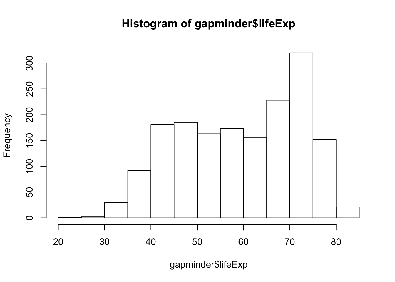

Version	Author	Date
61e3892	Anthony Hung	2020-06-23
20a6cfd	Anthony Hung	2020-04-30
310d040	Anthony Hung	2020-02-20
e02f5ce	Anthony Hung	2020-02-20
133df4a	Anthony Hung	2019-04-29

boxplot(lifeExp ~ continent, data = gapminder) #box plot for the life expectancies of all years per continent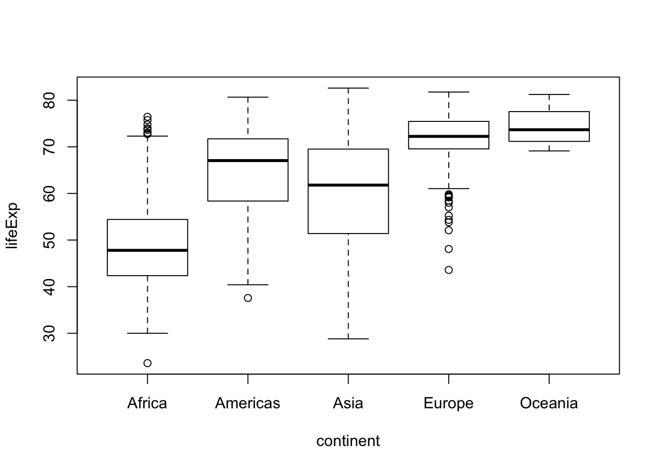

Version	Author	Date
61e3892	Anthony Hung	2020-06-23
20a6cfd	Anthony Hung	2020-04-30
310d040	Anthony Hung	2020-02-20
e02f5ce	Anthony Hung	2020-02-20
5a37a3e	Anthony Hung	2020-02-14
133df4a	Anthony Hung	2019-04-29

Setting a random seed

R has many functions that use a random number generator to generate an output. For example, the r____ functions (e.g. rbinom, runif) pull numbers from a probability distribution of your choice. In order to create reproducible analyses, it is often advantageous to be able to reliably obtain the same “random” number after running the same function over again. In order to do so, we can set a seed for the random number generator.

runif(1,0,1) #runif pulls a number from the uniform distribution with a set of given parameters

[1] 0.1944457

runif(1,0,1) #we can see that running runif twice gives you differnt results

[1] 0.205278

set.seed(1234) #setting a seed allows us to obtain reproducible results from functions that use the random number generator
runif(1,0,1)

[1] 0.1137034

set.seed(1234)
runif(1,0,1)

[1] 0.1137034

Reading and writing data in R

Finally, let us address probably one of the most important points when working with statistics in science: how to get the data you have collected into your R environment. For this part of the lesson, we will be working with the bandersnatch.csv file (created by Katie Long) located here: https://raw.githubusercontent.com/anthonyhung/MSTPsummerstatistics/master/data/bandersnatch.csv. If you would like to have your own copy of this dataset, you can open up a terminal window and run the commands (tools menu in R studio).

cd ~/Desktop
mkdir data
cd data
wget https://raw.githubusercontent.com/anthonyhung/MSTPsummerstatistics/master/data/bandersnatch.csv

Now that we have a copy of the data in a data directory on our desktop, we can load it into R using a relative or absolute directory path and the read.csv function.

data <- read.csv("~/Desktop/data/bandersnatch.csv")
#let's take a look at the dataset we've just loaded
head(data)

  Color  Fur Baseline.Frumiosity Post.Frumiosity
1   Red Nude            4.477127        11.46590
2   Red Nude            4.113727        11.09354
3   Red Nude            4.806221        11.81268
4   Red Nude            5.357348        12.36704
5   Red Nude            5.951754        12.96135
6   Red Nude            3.593995        10.62375

summary(data)

  Color           Fur         Baseline.Frumiosity Post.Frumiosity 
 Blue:200000   Furry:200000   Min.   :-1.108      Min.   : 1.887  
 Red :200000   Nude :200000   1st Qu.: 4.001      1st Qu.: 4.044  
                              Median : 6.980      Median : 8.976  
                              Mean   : 6.001      Mean   : 9.001  
                              3rd Qu.: 8.961      3rd Qu.:13.956  
                              Max.   : 9.174      Max.   :16.192

#what is the difference between these two function calls?
head(read.csv("~/Desktop/data/bandersnatch.csv", header = T))

  Color  Fur Baseline.Frumiosity Post.Frumiosity
1   Red Nude            4.477127        11.46590
2   Red Nude            4.113727        11.09354
3   Red Nude            4.806221        11.81268
4   Red Nude            5.357348        12.36704
5   Red Nude            5.951754        12.96135
6   Red Nude            3.593995        10.62375

head(read.csv("~/Desktop/data/bandersnatch.csv", header = F))

     V1   V2                  V3              V4
1 Color  Fur Baseline Frumiosity Post-Frumiosity
2   Red Nude         4.477127244     11.46590322
3   Red Nude         4.113726932     11.09353649
4   Red Nude         4.806220524     11.81268077
5   Red Nude         5.357347878     12.36703951
6   Red Nude         5.951754455     12.96134984

#let's look at the structure of the data
class(data)

[1] "data.frame"

class(data$Color)

[1] "factor"

class(data$Baseline.Frumiosity)

[1] "numeric"

#let's make some plots with the data
hist(data$Baseline.Frumiosity)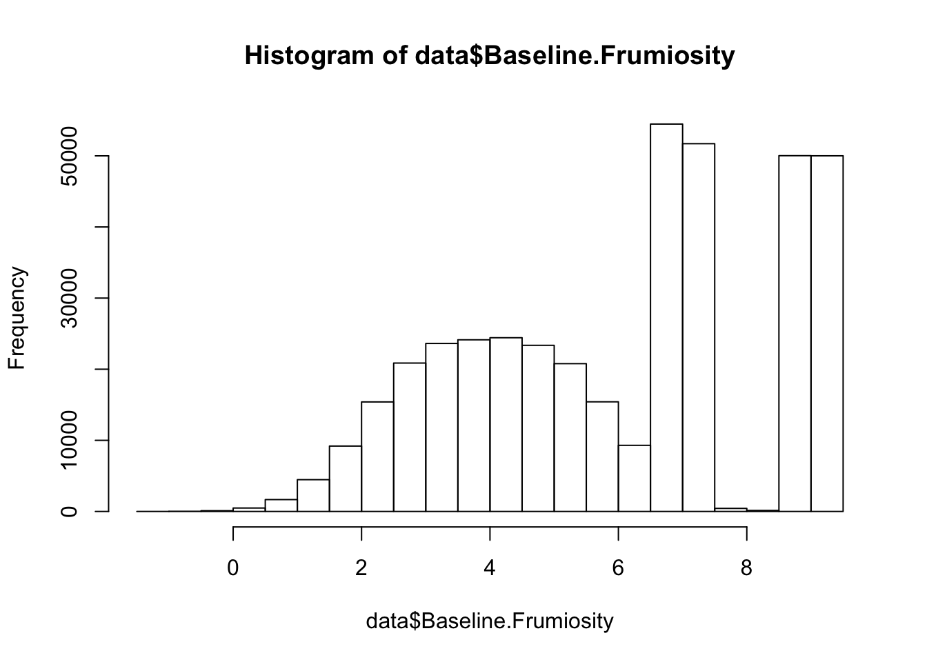

Version	Author	Date
61e3892	Anthony Hung	2020-06-23
20a6cfd	Anthony Hung	2020-04-30
310d040	Anthony Hung	2020-02-20
e02f5ce	Anthony Hung	2020-02-20
dd1e411	Anthony Hung	2019-05-22

hist(data$Post.Frumiosity)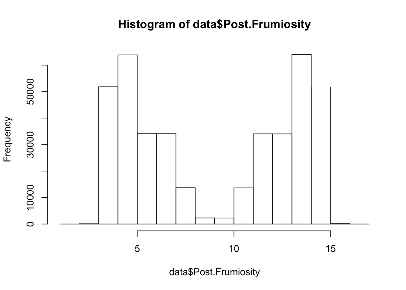

Version	Author	Date
61e3892	Anthony Hung	2020-06-23
20a6cfd	Anthony Hung	2020-04-30
310d040	Anthony Hung	2020-02-20
e02f5ce	Anthony Hung	2020-02-20
dd1e411	Anthony Hung	2019-05-22

plot(data$Baseline.Frumiosity, data$Post.Frumiosity)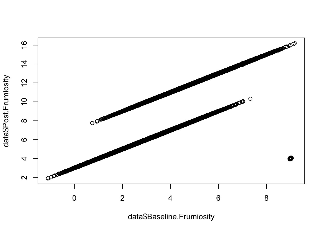

Version	Author	Date
61e3892	Anthony Hung	2020-06-23
20a6cfd	Anthony Hung	2020-04-30
310d040	Anthony Hung	2020-02-20
e02f5ce	Anthony Hung	2020-02-20
dd1e411	Anthony Hung	2019-05-22

#we can also write data files and export them using R
data$Size <- rnorm(nrow(data))
write.csv(data, "~/Desktop/data/new_bandersnatch.csv")

Exercises:

Write a function called calc_KE that takes as arguments the mass (in kg) and velocity (in m/s) of an object and returns the kinetic energy (in Joules) of an object. Use it to find the KE of a 0.5 kg rock moving at 1.2 m/s. 0.36 Joules
Working with the gapminder dataset, find the country with the highest life expectancy in 1962. Iceland

dplyr

The dplyr package is a powerful tool for working with dataframes (what is a dataframe?) in R. The framework of dplyr relies on the use of “pipes” or the “%>%” operator, to apply multiple useful functions to a dataframe sequentially. Today we will cover these functions:

mutate() adds new variables that are functions of existing variables select() picks variables based on their names. filter() picks cases based on their values. summarise() reduces multiple values down to a single summary. arrange() changes the ordering of the rows.

However, there are many more useful functions in the package that may come in handy depending on your specific problem!

library(dplyr)


Attaching package: 'dplyr'

The following objects are masked from 'package:stats':

    filter, lag

The following objects are masked from 'package:base':

    intersect, setdiff, setequal, union

gapminder

# A tibble: 1,704 x 6
   country     continent  year lifeExp      pop gdpPercap
   <fct>       <fct>     <int>   <dbl>    <int>     <dbl>
 1 Afghanistan Asia       1952    28.8  8425333      779.
 2 Afghanistan Asia       1957    30.3  9240934      821.
 3 Afghanistan Asia       1962    32.0 10267083      853.
 4 Afghanistan Asia       1967    34.0 11537966      836.
 5 Afghanistan Asia       1972    36.1 13079460      740.
 6 Afghanistan Asia       1977    38.4 14880372      786.
 7 Afghanistan Asia       1982    39.9 12881816      978.
 8 Afghanistan Asia       1987    40.8 13867957      852.
 9 Afghanistan Asia       1992    41.7 16317921      649.
10 Afghanistan Asia       1997    41.8 22227415      635.
# … with 1,694 more rows

#mutate
mutate(gapminder, GDP = gdpPercap * pop)

# A tibble: 1,704 x 7
   country     continent  year lifeExp      pop gdpPercap          GDP
   <fct>       <fct>     <int>   <dbl>    <int>     <dbl>        <dbl>
 1 Afghanistan Asia       1952    28.8  8425333      779.  6567086330.
 2 Afghanistan Asia       1957    30.3  9240934      821.  7585448670.
 3 Afghanistan Asia       1962    32.0 10267083      853.  8758855797.
 4 Afghanistan Asia       1967    34.0 11537966      836.  9648014150.
 5 Afghanistan Asia       1972    36.1 13079460      740.  9678553274.
 6 Afghanistan Asia       1977    38.4 14880372      786. 11697659231.
 7 Afghanistan Asia       1982    39.9 12881816      978. 12598563401.
 8 Afghanistan Asia       1987    40.8 13867957      852. 11820990309.
 9 Afghanistan Asia       1992    41.7 16317921      649. 10595901589.
10 Afghanistan Asia       1997    41.8 22227415      635. 14121995875.
# … with 1,694 more rows

gapminder %>% mutate(GDP = gdpPercap * pop) #pipes

# A tibble: 1,704 x 7
   country     continent  year lifeExp      pop gdpPercap          GDP
   <fct>       <fct>     <int>   <dbl>    <int>     <dbl>        <dbl>
 1 Afghanistan Asia       1952    28.8  8425333      779.  6567086330.
 2 Afghanistan Asia       1957    30.3  9240934      821.  7585448670.
 3 Afghanistan Asia       1962    32.0 10267083      853.  8758855797.
 4 Afghanistan Asia       1967    34.0 11537966      836.  9648014150.
 5 Afghanistan Asia       1972    36.1 13079460      740.  9678553274.
 6 Afghanistan Asia       1977    38.4 14880372      786. 11697659231.
 7 Afghanistan Asia       1982    39.9 12881816      978. 12598563401.
 8 Afghanistan Asia       1987    40.8 13867957      852. 11820990309.
 9 Afghanistan Asia       1992    41.7 16317921      649. 10595901589.
10 Afghanistan Asia       1997    41.8 22227415      635. 14121995875.
# … with 1,694 more rows

gapminder_with_GDP <- gapminder %>% mutate(GDP = gdpPercap * pop) #assign output to variable
gapminder_with_GDP

# A tibble: 1,704 x 7
   country     continent  year lifeExp      pop gdpPercap          GDP
   <fct>       <fct>     <int>   <dbl>    <int>     <dbl>        <dbl>
 1 Afghanistan Asia       1952    28.8  8425333      779.  6567086330.
 2 Afghanistan Asia       1957    30.3  9240934      821.  7585448670.
 3 Afghanistan Asia       1962    32.0 10267083      853.  8758855797.
 4 Afghanistan Asia       1967    34.0 11537966      836.  9648014150.
 5 Afghanistan Asia       1972    36.1 13079460      740.  9678553274.
 6 Afghanistan Asia       1977    38.4 14880372      786. 11697659231.
 7 Afghanistan Asia       1982    39.9 12881816      978. 12598563401.
 8 Afghanistan Asia       1987    40.8 13867957      852. 11820990309.
 9 Afghanistan Asia       1992    41.7 16317921      649. 10595901589.
10 Afghanistan Asia       1997    41.8 22227415      635. 14121995875.
# … with 1,694 more rows

#select
gapminder %>% select(c(country, continent, year))

# A tibble: 1,704 x 3
   country     continent  year
   <fct>       <fct>     <int>
 1 Afghanistan Asia       1952
 2 Afghanistan Asia       1957
 3 Afghanistan Asia       1962
 4 Afghanistan Asia       1967
 5 Afghanistan Asia       1972
 6 Afghanistan Asia       1977
 7 Afghanistan Asia       1982
 8 Afghanistan Asia       1987
 9 Afghanistan Asia       1992
10 Afghanistan Asia       1997
# … with 1,694 more rows

data %>% select(contains("frumiosity")) %>% slice(10)

  Baseline.Frumiosity Post.Frumiosity
1            4.894497        11.87147

gapminder %>%  select(starts_with("c"))

# A tibble: 1,704 x 2
   country     continent
   <fct>       <fct>    
 1 Afghanistan Asia     
 2 Afghanistan Asia     
 3 Afghanistan Asia     
 4 Afghanistan Asia     
 5 Afghanistan Asia     
 6 Afghanistan Asia     
 7 Afghanistan Asia     
 8 Afghanistan Asia     
 9 Afghanistan Asia     
10 Afghanistan Asia     
# … with 1,694 more rows

gapminder %>%  select(ends_with("p"))

# A tibble: 1,704 x 3
   lifeExp      pop gdpPercap
     <dbl>    <int>     <dbl>
 1    28.8  8425333      779.
 2    30.3  9240934      821.
 3    32.0 10267083      853.
 4    34.0 11537966      836.
 5    36.1 13079460      740.
 6    38.4 14880372      786.
 7    39.9 12881816      978.
 8    40.8 13867957      852.
 9    41.7 16317921      649.
10    41.8 22227415      635.
# … with 1,694 more rows

#filter
gapminder %>% filter(country == "United States")

# A tibble: 12 x 6
   country       continent  year lifeExp       pop gdpPercap
   <fct>         <fct>     <int>   <dbl>     <int>     <dbl>
 1 United States Americas   1952    68.4 157553000    13990.
 2 United States Americas   1957    69.5 171984000    14847.
 3 United States Americas   1962    70.2 186538000    16173.
 4 United States Americas   1967    70.8 198712000    19530.
 5 United States Americas   1972    71.3 209896000    21806.
 6 United States Americas   1977    73.4 220239000    24073.
 7 United States Americas   1982    74.6 232187835    25010.
 8 United States Americas   1987    75.0 242803533    29884.
 9 United States Americas   1992    76.1 256894189    32004.
10 United States Americas   1997    76.8 272911760    35767.
11 United States Americas   2002    77.3 287675526    39097.
12 United States Americas   2007    78.2 301139947    42952.

gapminder %>% filter(year > 1999)

# A tibble: 284 x 6
   country     continent  year lifeExp      pop gdpPercap
   <fct>       <fct>     <int>   <dbl>    <int>     <dbl>
 1 Afghanistan Asia       2002    42.1 25268405      727.
 2 Afghanistan Asia       2007    43.8 31889923      975.
 3 Albania     Europe     2002    75.7  3508512     4604.
 4 Albania     Europe     2007    76.4  3600523     5937.
 5 Algeria     Africa     2002    71.0 31287142     5288.
 6 Algeria     Africa     2007    72.3 33333216     6223.
 7 Angola      Africa     2002    41.0 10866106     2773.
 8 Angola      Africa     2007    42.7 12420476     4797.
 9 Argentina   Americas   2002    74.3 38331121     8798.
10 Argentina   Americas   2007    75.3 40301927    12779.
# … with 274 more rows

gapminder %>% filter()

# A tibble: 1,704 x 6
   country     continent  year lifeExp      pop gdpPercap
   <fct>       <fct>     <int>   <dbl>    <int>     <dbl>
 1 Afghanistan Asia       1952    28.8  8425333      779.
 2 Afghanistan Asia       1957    30.3  9240934      821.
 3 Afghanistan Asia       1962    32.0 10267083      853.
 4 Afghanistan Asia       1967    34.0 11537966      836.
 5 Afghanistan Asia       1972    36.1 13079460      740.
 6 Afghanistan Asia       1977    38.4 14880372      786.
 7 Afghanistan Asia       1982    39.9 12881816      978.
 8 Afghanistan Asia       1987    40.8 13867957      852.
 9 Afghanistan Asia       1992    41.7 16317921      649.
10 Afghanistan Asia       1997    41.8 22227415      635.
# … with 1,694 more rows

#summarise
gapminder %>% summarise(mean(gdpPercap))

# A tibble: 1 x 1
  `mean(gdpPercap)`
              <dbl>
1             7215.

#arrange
gapminder %>% arrange(year)

# A tibble: 1,704 x 6
   country     continent  year lifeExp      pop gdpPercap
   <fct>       <fct>     <int>   <dbl>    <int>     <dbl>
 1 Afghanistan Asia       1952    28.8  8425333      779.
 2 Albania     Europe     1952    55.2  1282697     1601.
 3 Algeria     Africa     1952    43.1  9279525     2449.
 4 Angola      Africa     1952    30.0  4232095     3521.
 5 Argentina   Americas   1952    62.5 17876956     5911.
 6 Australia   Oceania    1952    69.1  8691212    10040.
 7 Austria     Europe     1952    66.8  6927772     6137.
 8 Bahrain     Asia       1952    50.9   120447     9867.
 9 Bangladesh  Asia       1952    37.5 46886859      684.
10 Belgium     Europe     1952    68    8730405     8343.
# … with 1,694 more rows

gapminder %>% arrange(desc(year))

# A tibble: 1,704 x 6
   country     continent  year lifeExp       pop gdpPercap
   <fct>       <fct>     <int>   <dbl>     <int>     <dbl>
 1 Afghanistan Asia       2007    43.8  31889923      975.
 2 Albania     Europe     2007    76.4   3600523     5937.
 3 Algeria     Africa     2007    72.3  33333216     6223.
 4 Angola      Africa     2007    42.7  12420476     4797.
 5 Argentina   Americas   2007    75.3  40301927    12779.
 6 Australia   Oceania    2007    81.2  20434176    34435.
 7 Austria     Europe     2007    79.8   8199783    36126.
 8 Bahrain     Asia       2007    75.6    708573    29796.
 9 Bangladesh  Asia       2007    64.1 150448339     1391.
10 Belgium     Europe     2007    79.4  10392226    33693.
# … with 1,694 more rows

gapminder %>% arrange(country, desc(year))

# A tibble: 1,704 x 6
   country     continent  year lifeExp      pop gdpPercap
   <fct>       <fct>     <int>   <dbl>    <int>     <dbl>
 1 Afghanistan Asia       2007    43.8 31889923      975.
 2 Afghanistan Asia       2002    42.1 25268405      727.
 3 Afghanistan Asia       1997    41.8 22227415      635.
 4 Afghanistan Asia       1992    41.7 16317921      649.
 5 Afghanistan Asia       1987    40.8 13867957      852.
 6 Afghanistan Asia       1982    39.9 12881816      978.
 7 Afghanistan Asia       1977    38.4 14880372      786.
 8 Afghanistan Asia       1972    36.1 13079460      740.
 9 Afghanistan Asia       1967    34.0 11537966      836.
10 Afghanistan Asia       1962    32.0 10267083      853.
# … with 1,694 more rows

#putting it all together. what if we wanted to know the highest absolute GDP of Zimbabwe between 1982 and 2007? (printing out only 1 value)
gapminder %>% 
  mutate(GDP = gdpPercap * pop) %>% 
  filter(country == "Zimbabwe", between(year, 1982, 2007)) %>% #between!
  arrange(desc(GDP)) %>% 
  select(GDP) %>% 
  top_n(1)

Selecting by GDP

# A tibble: 1 x 1
          GDP
        <dbl>
1 9037850590.

# what if we wanted the average GDP of Zimbabwe between 1982 and 2007?
gapminder %>% 
  mutate(GDP = gdpPercap * pop) %>% 
  filter(country == "Zimbabwe", between(year, 1982, 2007)) %>% #between!
  summarise(mean(GDP))

# A tibble: 1 x 1
  `mean(GDP)`
        <dbl>
1 7131763852.

#Bonus: group_by
gapminder %>% 
  group_by(country) %>% 
  summarise(mean(gdpPercap))

# A tibble: 142 x 2
   country     `mean(gdpPercap)`
   <fct>                   <dbl>
 1 Afghanistan              803.
 2 Albania                 3255.
 3 Algeria                 4426.
 4 Angola                  3607.
 5 Argentina               8956.
 6 Australia              19981.
 7 Austria                20412.
 8 Bahrain                18078.
 9 Bangladesh               818.
10 Belgium                19901.
# … with 132 more rows

gapminder %>% 
  group_by(continent) %>% 
  filter(year == "2007") %>% 
  summarise(n())

# A tibble: 5 x 2
  continent `n()`
  <fct>     <int>
1 Africa       52
2 Americas     25
3 Asia         33
4 Europe       30
5 Oceania       2

Exercise: Using dplyr functions, find the Country in Asia that had the largest population in 1982 and tell me it’s total GDP that year.

Exercise: The labs data contains information about labs taken for patients over a period of time. Using dplyr, compute the ratio of PaO2/FiO2 for each patient at each time point and output a table of the minimum recorded PaO2/FiO2 ratio for each patient in the data. (not very useful but necessary hint: what is the difference between “PAO2” and “PO2 (ARTERIAL)”?)

labs <- read.csv("data/labs.csv")

Handy cheat sheets

https://rstudio.com/wp-content/uploads/2016/10/r-cheat-sheet-3.pdf https://rstudio.com/wp-content/uploads/2015/02/data-wrangling-cheatsheet.pdf

sessionInfo()

R version 3.6.3 (2020-02-29)
Platform: x86_64-apple-darwin15.6.0 (64-bit)
Running under: macOS Catalina 10.15.5

Matrix products: default
BLAS:   /Library/Frameworks/R.framework/Versions/3.6/Resources/lib/libRblas.0.dylib
LAPACK: /Library/Frameworks/R.framework/Versions/3.6/Resources/lib/libRlapack.dylib

locale:
[1] en_US.UTF-8/en_US.UTF-8/en_US.UTF-8/C/en_US.UTF-8/en_US.UTF-8

attached base packages:
[1] stats     graphics  grDevices utils     datasets  methods   base     

other attached packages:
[1] dplyr_0.8.5     gapminder_0.3.0

loaded via a namespace (and not attached):
 [1] Rcpp_1.0.4.6     knitr_1.26       whisker_0.4      magrittr_1.5    
 [5] workflowr_1.5.0  tidyselect_1.0.0 R6_2.4.1         rlang_0.4.5     
 [9] fansi_0.4.1      stringr_1.4.0    tools_3.6.3      xfun_0.12       
[13] utf8_1.1.4       cli_2.0.2        git2r_0.26.1     htmltools_0.4.0 
[17] ellipsis_0.3.0   assertthat_0.2.1 yaml_2.2.1       digest_0.6.25   
[21] rprojroot_1.3-2  tibble_3.0.1     lifecycle_0.2.0  crayon_1.3.4    
[25] purrr_0.3.4      later_1.0.0      vctrs_0.2.4      promises_1.1.0  
[29] fs_1.3.1         glue_1.4.0       evaluate_0.14    rmarkdown_1.18  
[33] stringi_1.4.5    compiler_3.6.3   pillar_1.4.3     backports_1.1.6 
[37] httpuv_1.5.2     pkgconfig_2.0.3

Introduction to R

Anthony Hung

2019-04-25