Normalization and filtering of bulkRNAseq data
Anthony Hung
2021-01-19
Last updated: 2021-01-21
Checks: 7 0
Knit directory: invitroOA_pilot_repository/
This reproducible R Markdown analysis was created with workflowr (version 1.6.2). The Checks tab describes the reproducibility checks that were applied when the results were created. The Past versions tab lists the development history.
Great! Since the R Markdown file has been committed to the Git repository, you know the exact version of the code that produced these results.
Great job! The global environment was empty. Objects defined in the global environment can affect the analysis in your R Markdown file in unknown ways. For reproduciblity it’s best to always run the code in an empty environment.
The command set.seed(20210119) was run prior to running the code in the R Markdown file. Setting a seed ensures that any results that rely on randomness, e.g. subsampling or permutations, are reproducible.
Great job! Recording the operating system, R version, and package versions is critical for reproducibility.
Nice! There were no cached chunks for this analysis, so you can be confident that you successfully produced the results during this run.
Great job! Using relative paths to the files within your workflowr project makes it easier to run your code on other machines.
Great! You are using Git for version control. Tracking code development and connecting the code version to the results is critical for reproducibility.
The results in this page were generated with repository version 78cfbcd. See the Past versions tab to see a history of the changes made to the R Markdown and HTML files.
Note that you need to be careful to ensure that all relevant files for the analysis have been committed to Git prior to generating the results (you can use wflow_publish or wflow_git_commit). workflowr only checks the R Markdown file, but you know if there are other scripts or data files that it depends on. Below is the status of the Git repository when the results were generated:
Ignored files:
    Ignored:    .DS_Store
    Ignored:    .Rhistory
    Ignored:    .Rproj.user/
    Ignored:    data/.DS_Store
    Ignored:    data/external_scRNA/.DS_Store

Unstaged changes:
    Deleted:    analysis/figure/powerAnalysis.Rmd/curve-1.png
    Deleted:    analysis/figure/powerAnalysis.Rmd/hypoxia-1.png
    Deleted:    analysis/figure/powerAnalysis.Rmd/hypoxia-2.png
    Deleted:    analysis/figure/powerAnalysis.Rmd/hypoxia-3.png
    Deleted:    analysis/figure/powerAnalysis.Rmd/hypoxia-4.png
    Deleted:    analysis/figure/powerAnalysis.Rmd/hypoxia-5.png
    Deleted:    analysis/figure/powerAnalysis.Rmd/hypoxia-6.png
    Deleted:    analysis/figure/powerAnalysis.Rmd/hypoxia-7.png
    Deleted:    analysis/figure/powerAnalysis.Rmd/hypoxia-8.png
Note that any generated files, e.g. HTML, png, CSS, etc., are not included in this status report because it is ok for generated content to have uncommitted changes.
These are the previous versions of the repository in which changes were made to the R Markdown (analysis/normFilter_bulkRNA.Rmd) and HTML (docs/normFilter_bulkRNA.html) files. If you’ve configured a remote Git repository (see ?wflow_git_remote), click on the hyperlinks in the table below to view the files as they were in that past version.
| File | Version | Author | Date | Message |
|---|---|---|---|---|
| Rmd | e3fbd0f | Anthony Hung | 2021-01-21 | add ward et al data files to data |
| html | e3fbd0f | Anthony Hung | 2021-01-21 | add ward et al data files to data |
| Rmd | 0711682 | Anthony Hung | 2021-01-21 | start normalization file |
| html | 0711682 | Anthony Hung | 2021-01-21 | start normalization file |
| Rmd | 28f57fa | Anthony Hung | 2021-01-19 | Add files for analysis |
Introduction
This code takes the raw count data from bulk RNA sequencing and performs upper quartile normalziation on the data, filtering out lowly expressed genes. It then saves the resulting data and filtered count data (unnormalized) as R objects.
Here we also plot PCA plots to visualize the structure of the full data set (PCA plots for the data set excluding the sample that failed QC are located in the Modeling and removing unwanted technical variation page).
Load data and libraries
Here we are loading both the full data and the data without the one sample that failed QC.
library("gplots")
Attaching package: 'gplots'The following object is masked from 'package:stats':
lowesslibrary("ggplot2")
library("reshape")
library("edgeR")Loading required package: limmalibrary("RColorBrewer")
library("scales")
library("cowplot")
Attaching package: 'cowplot'The following object is masked from 'package:reshape':
stamptheme_set(theme_cowplot())
library("dplyr")
Attaching package: 'dplyr'The following object is masked from 'package:reshape':
renameThe following objects are masked from 'package:stats':
filter, lagThe following objects are masked from 'package:base':
intersect, setdiff, setequal, union# Load colors
colors <- colorRampPalette(c(brewer.pal(9, "Blues")[1],brewer.pal(9, "Blues")[9]))(100)
pal <- c(brewer.pal(9, "Set1"), brewer.pal(8, "Set2"), brewer.pal(12, "Set3"))
# load in relabeled counts
raw_counts <- readRDS("data/raw_counts_relabeled.rds")
raw_counts_includeNA19160 <- readRDS("data/raw_counts_relabeled_includeNA19160.rds")
# Create DGEList object to allow for easier application of different normalization methods
raw_counts <- DGEList(raw_counts, group = colnames(raw_counts))
raw_counts_includeNA19160 <- DGEList(raw_counts_includeNA19160, group = colnames(raw_counts_includeNA19160))
# load in reordered sample information
sampleinfo <- readRDS("data/Sample.info.RNAseq.reordered.rds")
sampleinfo_includeNA19160 <- readRDS("data/Sample.info.RNAseq.reordered_includeNA19160.rds")Upperquartile Normalization
Apply upperquartile normalization to the data.
upperquartile <- calcNormFactors(raw_counts, method = "upperquartile")
upperquartile <- cpm(upperquartile, log=TRUE, normalized.lib.sizes = T)
head(upperquartile)
18855_3_S 19160_3_S 18856_3_U 18856_1_U 18855_2_S 18856_2_S
ENSG00000223972 -3.129986 -3.129986 -3.129986 -3.129986 -3.129986 -3.129986
ENSG00000227232 -1.376624 -2.046788 -2.154778 -2.585632 -2.545595 -1.167335
ENSG00000278267 -3.129986 -3.129986 -3.129986 -3.129986 -3.129986 -3.129986
ENSG00000243485 -3.129986 -3.129986 -3.129986 -3.129986 -3.129986 -3.129986
ENSG00000284332 -3.129986 -3.129986 -3.129986 -3.129986 -3.129986 -3.129986
ENSG00000237613 -3.129986 -3.129986 -3.129986 -3.129986 -3.129986 -3.129986
19160_3_U 18855_2_U 19160_2_S 18855_1_S 18856_1_S 19160_1_S
ENSG00000223972 -3.129986 -3.129986 -3.129986 -3.129986 -3.129986 -3.129986
ENSG00000227232 -3.129986 -2.527469 -1.317333 -1.415729 -3.129986 -2.313104
ENSG00000278267 -3.129986 -3.129986 -3.129986 -3.129986 -3.129986 -3.129986
ENSG00000243485 -3.129986 -3.129986 -3.129986 -3.129986 -3.129986 -3.129986
ENSG00000284332 -3.129986 -3.129986 -3.129986 -3.129986 -3.129986 -3.129986
ENSG00000237613 -3.129986 -3.129986 -3.129986 -3.129986 -3.129986 -3.129986
19160_2_U 18855_1_U 18856_3_S 18856_2_U 18855_3_U
ENSG00000223972 -3.129986 -3.129986 -3.129986 -3.129986 -3.129986
ENSG00000227232 -2.601918 -1.247154 -2.084127 -1.609909 -3.129986
ENSG00000278267 -3.129986 -3.129986 -3.129986 -3.129986 -3.129986
ENSG00000243485 -3.129986 -3.129986 -3.129986 -3.129986 -3.129986
ENSG00000284332 -3.129986 -3.129986 -3.129986 -3.129986 -3.129986
ENSG00000237613 -3.129986 -3.129986 -3.129986 -3.129986 -3.129986strained <- sampleinfo$treatment == "Strain"
unstrained <- sampleinfo$treatment == "Unstrain"
ind_1 <- sampleinfo$Individual == "NA18855 "
ind_2 <- sampleinfo$Individual == "NA18856 "
ind_3 <- sampleinfo$Individual == "NA19160 "
# Look at density plots for all individuals broken down by each treatment type
col = as.data.frame(pal[as.numeric(sampleinfo$Individual)])
plotDensities(upperquartile[,strained], col=col[strained, ], legend="topright")
| Version | Author | Date |
|---|---|---|
| 0711682 | Anthony Hung | 2021-01-21 |
plotDensities(upperquartile[,unstrained], col=col[unstrained, ], legend="topright")
| Version | Author | Date |
|---|---|---|
| 0711682 | Anthony Hung | 2021-01-21 |
# Look at density plots broken down by individual
col = as.data.frame(pal[as.numeric(sampleinfo$treatment)])

plotDensities(upperquartile[,ind_1], col=col[ind_1, ], legend="topright")
| Version | Author | Date |
|---|---|---|
| 0711682 | Anthony Hung | 2021-01-21 |
plotDensities(upperquartile[,ind_2], col=col[ind_2, ], legend="topright")
| Version | Author | Date |
|---|---|---|
| 0711682 | Anthony Hung | 2021-01-21 |
plotDensities(upperquartile[,ind_3], col=col[ind_3, ], legend="topright")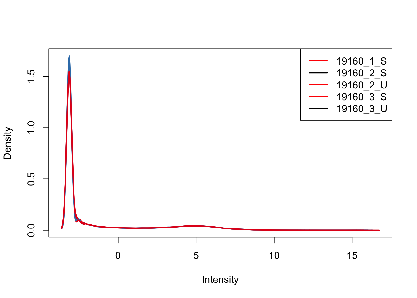
| Version | Author | Date |
|---|---|---|
| 0711682 | Anthony Hung | 2021-01-21 |
Boxplots of upperquartile across samples
meltupperquartile <- melt(upperquartile)
names(meltupperquartile) <- c("gene", "sampleID", "upperquartile")
p <- ggplot(meltupperquartile, aes(factor(sampleID), upperquartile))
p + geom_boxplot() + theme(axis.text.x = element_text(angle = 90))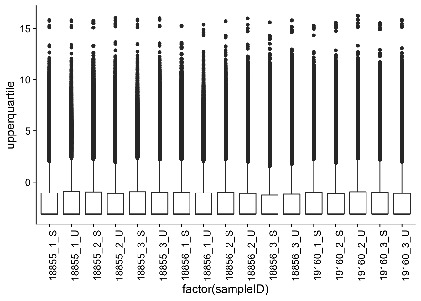
| Version | Author | Date |
|---|---|---|
| 0711682 | Anthony Hung | 2021-01-21 |
Filtering for lowly expressed genes
The criteria we are using is an average log2upperquartile > 2.5 in at least 4 samples. After this filtering step, 10486 genes remain.
cutoff <- 2.5

keep <- rowSums( upperquartile > cutoff ) >=4

counts_upperquartile <- raw_counts[keep,]
filtered_upperquartile <- upperquartile[keep,]
dim(filtered_upperquartile)
[1] 10486 17Boxplots of normalized+filtered counts across samples
After normalization, the data do indeed look more normal than when unnormalized.
melt_filt_upperquartile <- melt(filtered_upperquartile)
names(melt_filt_upperquartile) <- c("gene", "sampleID", "log2upperquartile")
p1 <- ggplot(melt_filt_upperquartile, aes(factor(sampleID), log2upperquartile))
p1 + geom_boxplot() + theme(axis.text.x = element_text(angle = 90))
| Version | Author | Date |
|---|---|---|
| 0711682 | Anthony Hung | 2021-01-21 |
plotDensities(filtered_upperquartile, legend = F)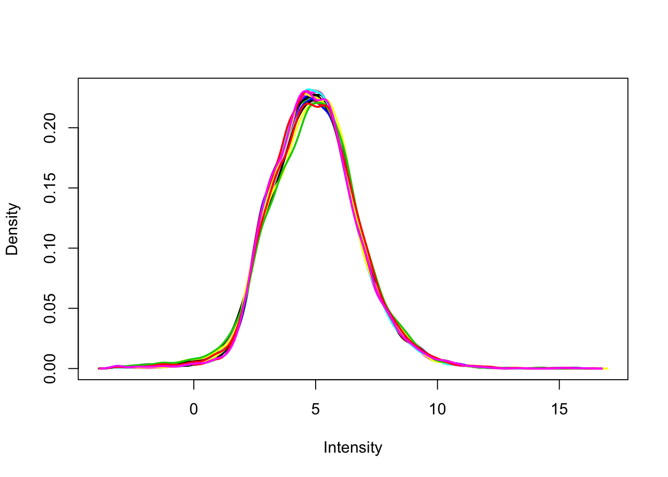
| Version | Author | Date |
|---|---|---|
| 0711682 | Anthony Hung | 2021-01-21 |
Save normalized/filtered count matrix and filtered count matrix
saveRDS(counts_upperquartile, "data/filtered_counts.rds")
saveRDS(filtered_upperquartile, "data/norm_filtered_counts.rds")
PCA plots for dataset including the sample filtered out by QC
upperquartile Normalization of full data
upperquartile_includeNA19160 <- calcNormFactors(raw_counts_includeNA19160, method = "upperquartile")
upperquartile_includeNA19160 <- cpm(upperquartile_includeNA19160, log=TRUE, normalized.lib.sizes = T)
head(upperquartile_includeNA19160)
18855_3_S 19160_3_S 18856_3_U 18856_1_U 18855_2_S 18856_2_S
ENSG00000223972 -3.101145 -3.101145 -3.101145 -3.101145 -3.101145 -3.101145
ENSG00000227232 -1.371277 -2.027812 -2.134933 -2.565487 -2.526602 -1.157511
ENSG00000278267 -3.101145 -3.101145 -3.101145 -3.101145 -3.101145 -3.101145
ENSG00000243485 -3.101145 -3.101145 -3.101145 -3.101145 -3.101145 -3.101145
ENSG00000284332 -3.101145 -3.101145 -3.101145 -3.101145 -3.101145 -3.101145
ENSG00000237613 -3.101145 -3.101145 -3.101145 -3.101145 -3.101145 -3.101145
19160_3_U 18855_2_U 19160_2_S 18855_1_S 18856_1_S 19160_1_S
ENSG00000223972 -3.101145 -3.101145 -3.101145 -3.101145 -3.101145 -3.101145
ENSG00000227232 -3.101145 -2.508875 -1.294699 -1.401586 -3.101145 -2.296780
ENSG00000278267 -3.101145 -3.101145 -3.101145 -3.101145 -3.101145 -3.101145
ENSG00000243485 -3.101145 -3.101145 -3.101145 -3.101145 -3.101145 -3.101145
ENSG00000284332 -3.101145 -3.101145 -3.101145 -3.101145 -3.101145 -3.101145
ENSG00000237613 -3.101145 -3.101145 -3.101145 -3.101145 -3.101145 -3.101145
19160_2_U 19160_1_U 18855_1_U 18856_3_S 18856_2_U 18855_3_U
ENSG00000223972 -3.101145 -3.101145 -3.101145 -3.101145 -3.101145 -3.101145
ENSG00000227232 -2.577970 -2.336134 -1.239235 -2.062052 -1.601659 -3.101145
ENSG00000278267 -3.101145 -3.101145 -3.101145 -3.101145 -3.101145 -3.101145
ENSG00000243485 -3.101145 -3.101145 -3.101145 -3.101145 -3.101145 -3.101145
ENSG00000284332 -3.101145 -3.101145 -3.101145 -3.101145 -3.101145 -3.101145
ENSG00000237613 -3.101145 -3.101145 -3.101145 -3.101145 -3.101145 -3.101145strained <- sampleinfo_includeNA19160$treatment == "Strain"
unstrained <- sampleinfo_includeNA19160$treatment == "Unstrain"
ind_1 <- sampleinfo_includeNA19160$Individual == "NA18855 "
ind_2 <- sampleinfo_includeNA19160$Individual == "NA18856 "
ind_3 <- sampleinfo_includeNA19160$Individual == "NA19160 "
# Look at density plots for all individuals broken down by each treatment type
col = as.data.frame(pal[as.numeric(sampleinfo_includeNA19160$Individual)])
plotDensities(upperquartile_includeNA19160[,strained], col=col[strained, ], legend="topright")
| Version | Author | Date |
|---|---|---|
| e3fbd0f | Anthony Hung | 2021-01-21 |
plotDensities(upperquartile_includeNA19160[,unstrained], col=col[unstrained, ], legend="topright")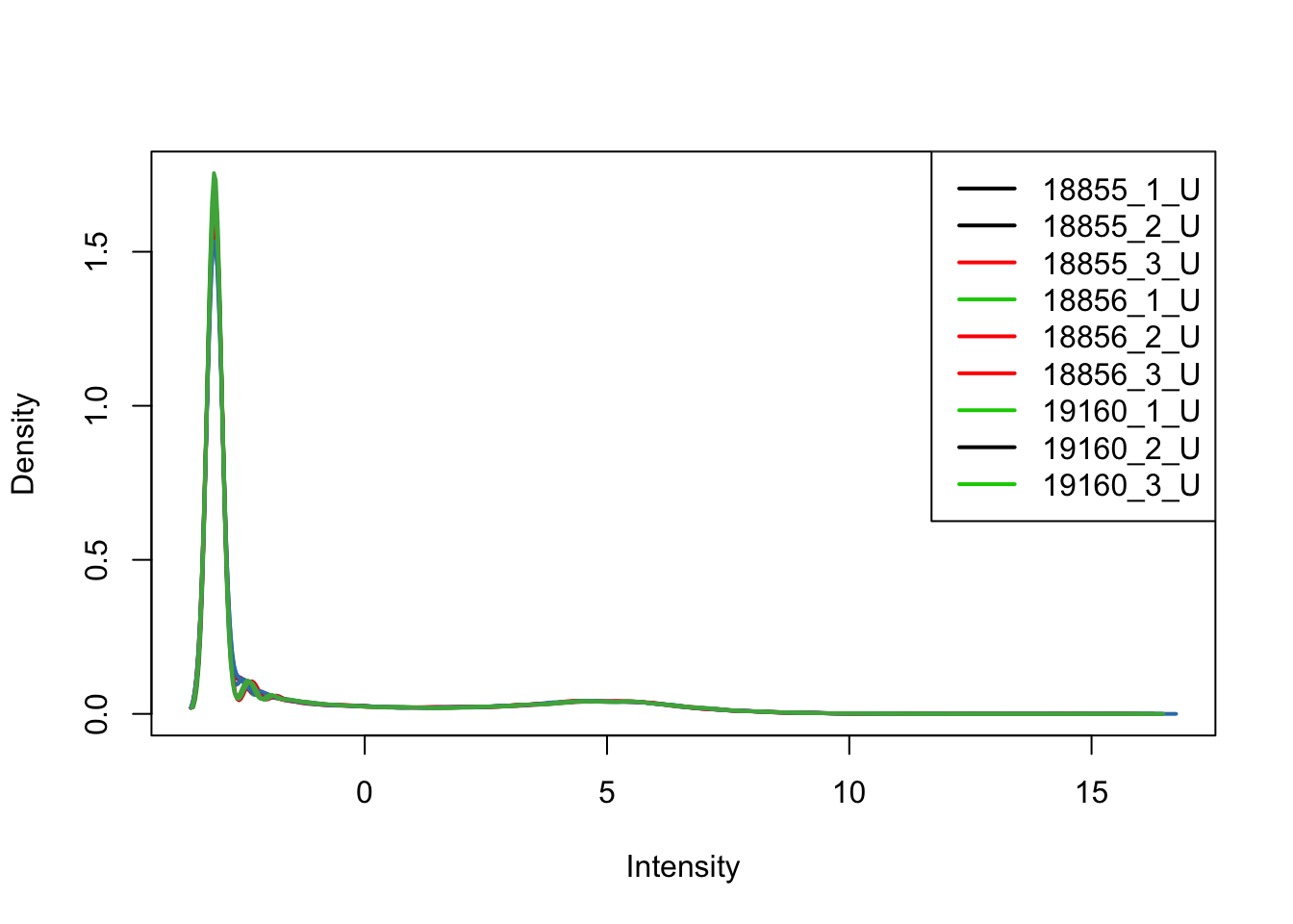
| Version | Author | Date |
|---|---|---|
| e3fbd0f | Anthony Hung | 2021-01-21 |
# Look at density plots broken down by individual
col = as.data.frame(pal[as.numeric(sampleinfo_includeNA19160$treatment)])

plotDensities(upperquartile_includeNA19160[,ind_1], col=col[ind_1, ], legend="topright")
| Version | Author | Date |
|---|---|---|
| e3fbd0f | Anthony Hung | 2021-01-21 |
plotDensities(upperquartile_includeNA19160[,ind_2], col=col[ind_2, ], legend="topright")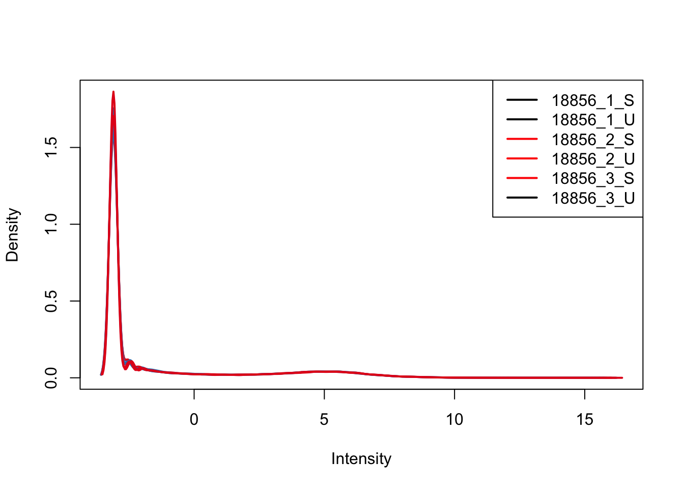
| Version | Author | Date |
|---|---|---|
| e3fbd0f | Anthony Hung | 2021-01-21 |
plotDensities(upperquartile_includeNA19160[,ind_3], col=col[ind_3, ], legend="topright")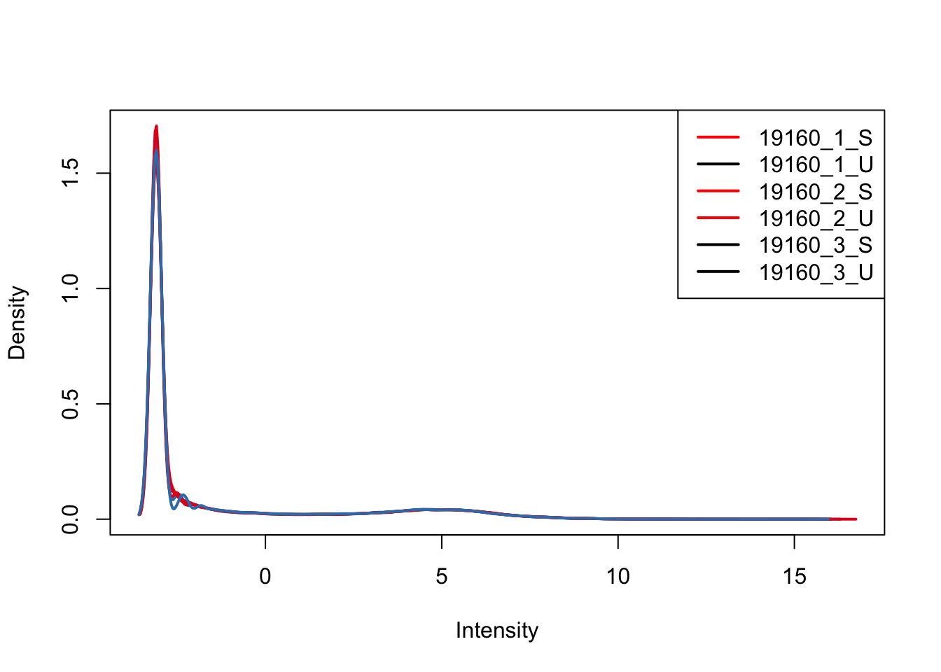
| Version | Author | Date |
|---|---|---|
| e3fbd0f | Anthony Hung | 2021-01-21 |
Boxplots of upperquartile across samples
meltupperquartile_includeNA19160 <- melt(upperquartile_includeNA19160)
names(meltupperquartile_includeNA19160) <- c("gene", "sampleID", "upperquartile")
p <- ggplot(meltupperquartile_includeNA19160, aes(factor(sampleID), upperquartile_includeNA19160))
p + geom_boxplot() + theme(axis.text.x = element_text(angle = 90))
| Version | Author | Date |
|---|---|---|
| e3fbd0f | Anthony Hung | 2021-01-21 |
Filtering for lowly expressed genes (avg log2upperquartile > 2.5 in at least 4 samples)
cutoff <- 2.5

keep <- rowSums( upperquartile_includeNA19160 > cutoff ) >=4

counts_upperquartile_includeNA19160 <- raw_counts_includeNA19160[keep,]
filtered_upperquartile_includeNA19160 <- upperquartile_includeNA19160[keep,]
dim(filtered_upperquartile_includeNA19160)
[1] 10517 18Boxplots of normalized+filtered counts across samples
melt_filt_upperquartile_includeNA19160 <- melt(filtered_upperquartile_includeNA19160)
names(melt_filt_upperquartile_includeNA19160) <- c("gene", "sampleID", "log2upperquartile")
p1 <- ggplot(melt_filt_upperquartile_includeNA19160, aes(factor(sampleID), log2upperquartile))
p1 + geom_boxplot() + theme(axis.text.x = element_text(angle = 90))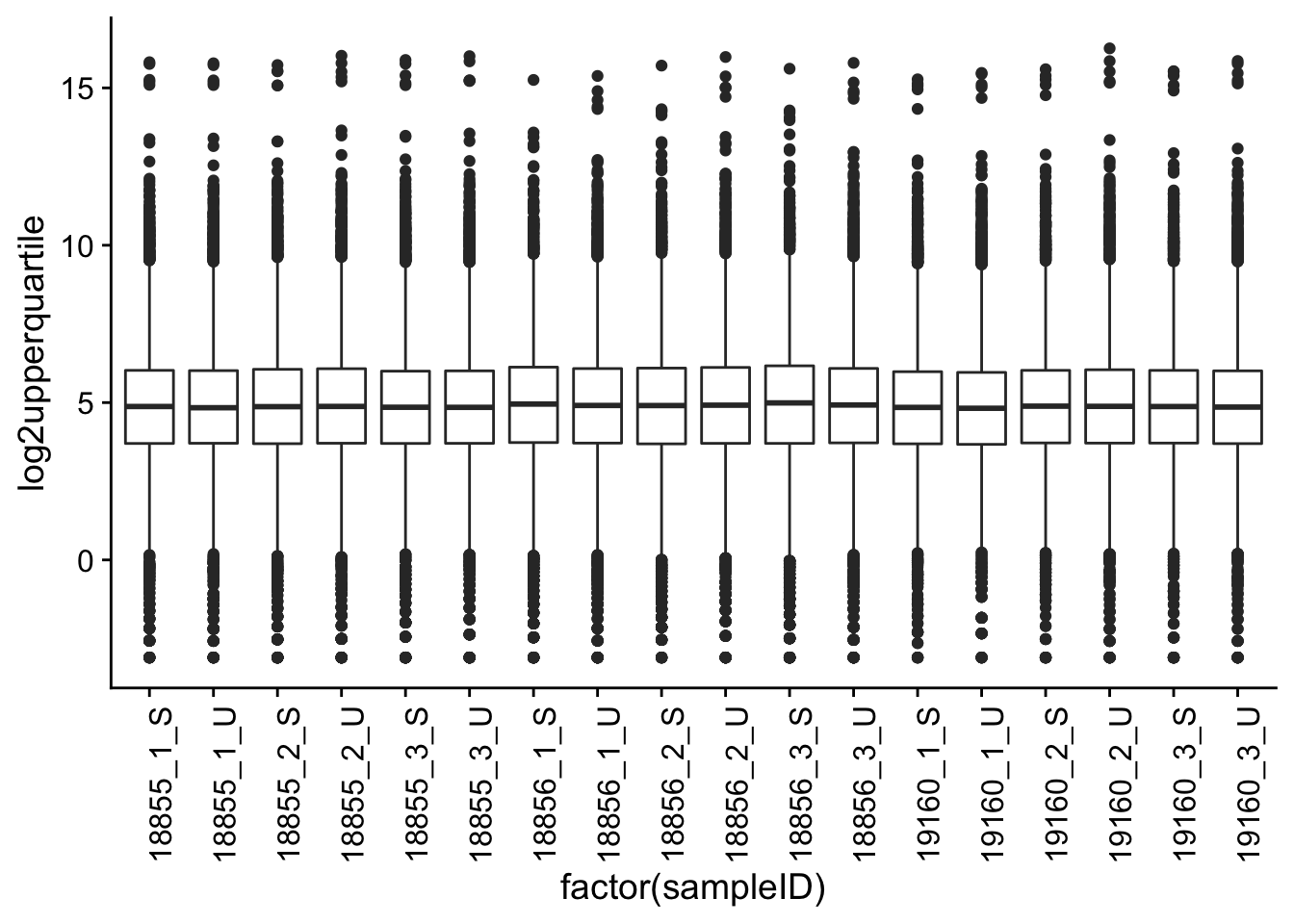
| Version | Author | Date |
|---|---|---|
| e3fbd0f | Anthony Hung | 2021-01-21 |
plotDensities(filtered_upperquartile_includeNA19160, legend = F)
| Version | Author | Date |
|---|---|---|
| e3fbd0f | Anthony Hung | 2021-01-21 |
Plot PCA
Reassuringly, the sample that was removed for low numbers of mapped reads still clusters as expected with its technical replicates.
#Load PCA plotting Function
source("code/PCA_fn.R")

# Perform PCA
pca_genes <- prcomp(t(filtered_upperquartile_includeNA19160), scale = T)
scores <- pca_genes$x

variances <- pca_genes$sdev^2
explained <- variances / sum(variances)
plot(pca_genes, main = "Variance per PC")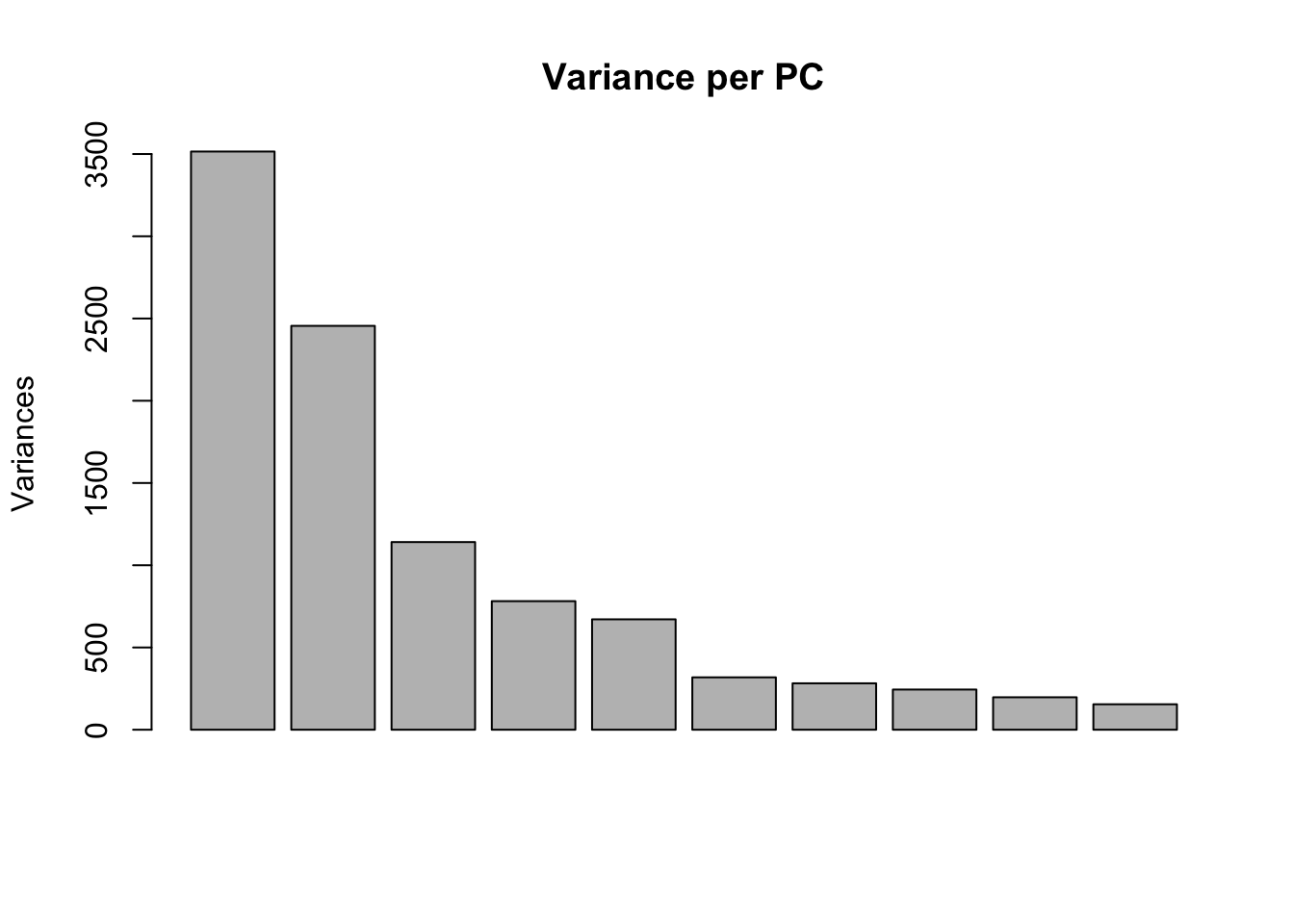
| Version | Author | Date |
|---|---|---|
| e3fbd0f | Anthony Hung | 2021-01-21 |
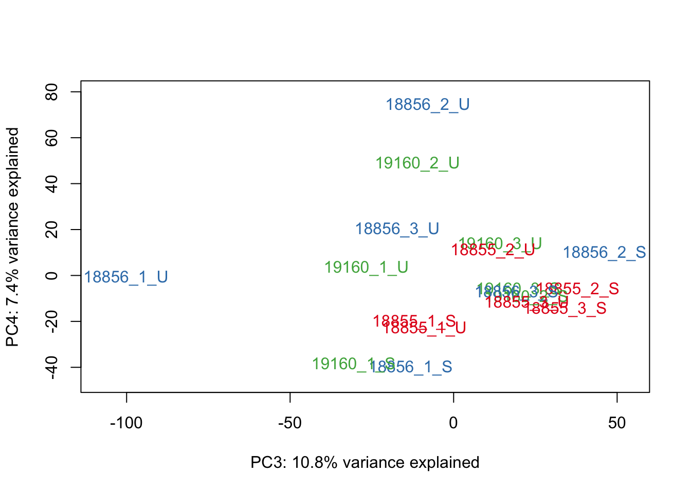
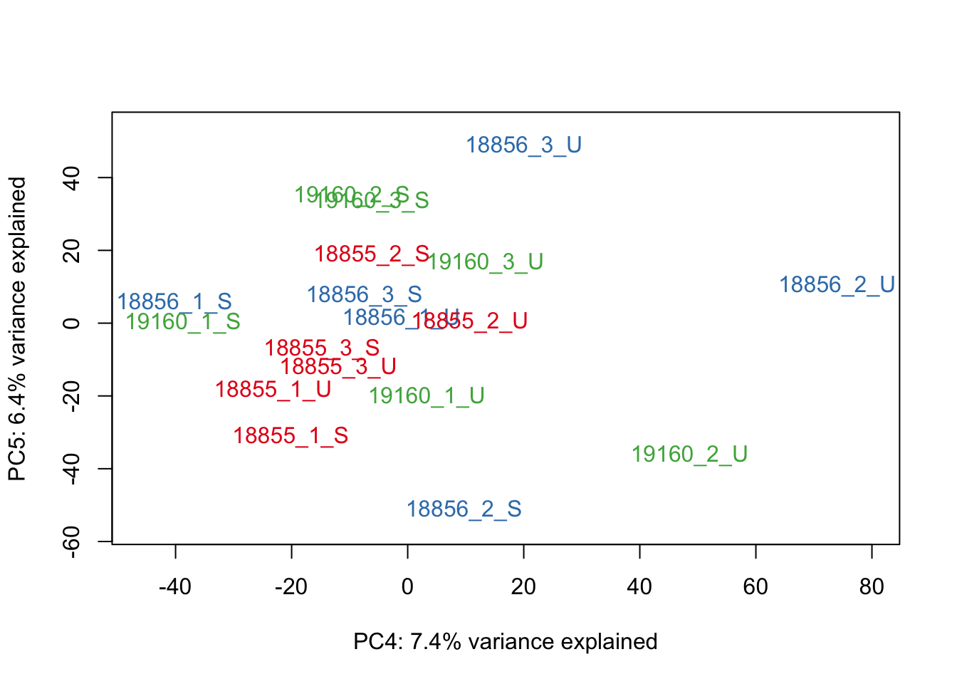
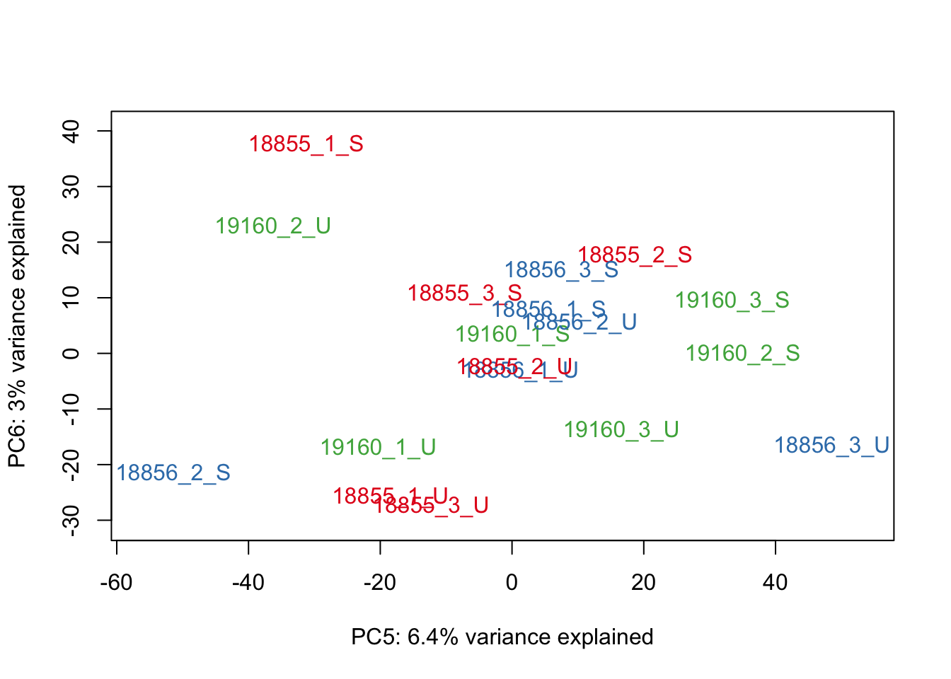
#Make PCA plots with the factors colored by Individual

### PCA norm+filt Data
for (n in 1:5){
  col.v <- pal[as.integer(sampleinfo_includeNA19160$Individual)]
  plot_scores(pca_genes, scores, n, n+1, col.v)
}
| Version | Author | Date |
|---|---|---|
| e3fbd0f | Anthony Hung | 2021-01-21 |

| Version | Author | Date |
|---|---|---|
| e3fbd0f | Anthony Hung | 2021-01-21 |
| Version | Author | Date |
|---|---|---|
| e3fbd0f | Anthony Hung | 2021-01-21 |
| Version | Author | Date |
|---|---|---|
| e3fbd0f | Anthony Hung | 2021-01-21 |
| Version | Author | Date |
|---|---|---|
| e3fbd0f | Anthony Hung | 2021-01-21 |
#make PCA plots with symbols as treatment status and colors as individuals for figure
library(ggfortify)
autoplot(pca_genes, data = sampleinfo_includeNA19160, colour = "Individual", shape = "treatment", size = 3) +
     theme_cowplot() +
     theme(legend.position = "none")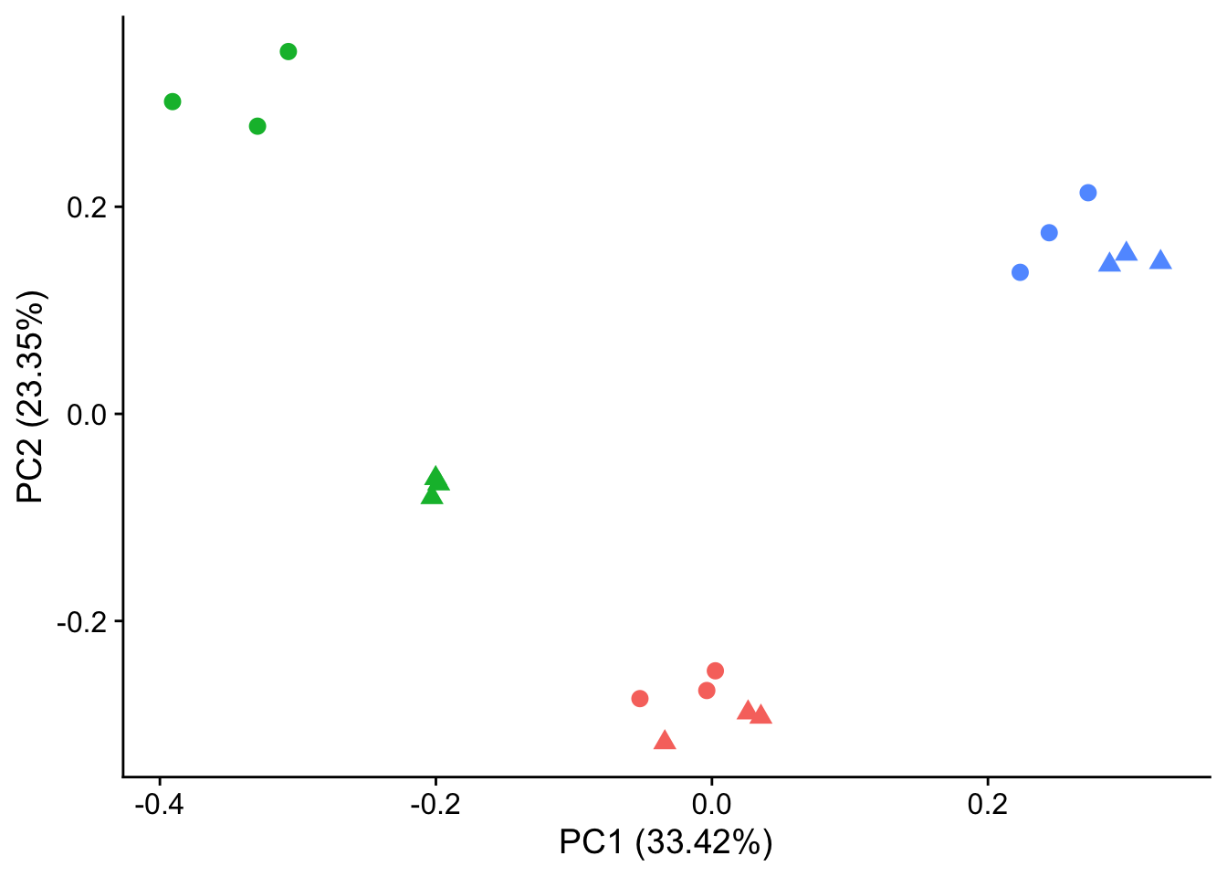
| Version | Author | Date |
|---|---|---|
| e3fbd0f | Anthony Hung | 2021-01-21 |
autoplot(pca_genes, data = sampleinfo_includeNA19160, colour = "Individual", shape = "treatment") +
     theme_cowplot()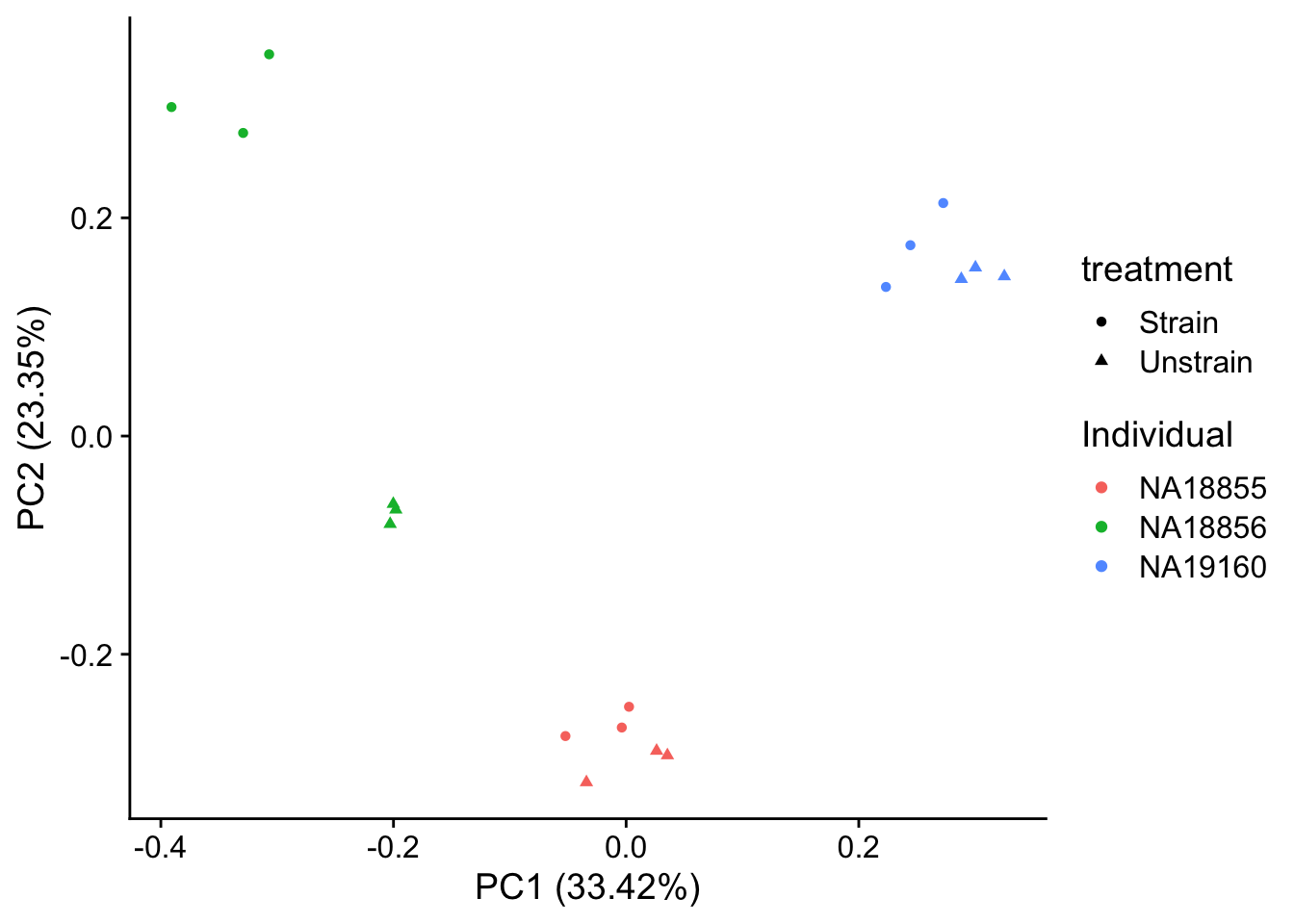
| Version | Author | Date |
|---|---|---|
| e3fbd0f | Anthony Hung | 2021-01-21 |
autoplot(pca_genes, data = sampleinfo_includeNA19160, colour = "Individual", shape = "treatment", size = 3, x = 3, y = 4) +
     theme_cowplot() +
     theme(legend.position = "none")
| Version | Author | Date |
|---|---|---|
| e3fbd0f | Anthony Hung | 2021-01-21 |
autoplot(pca_genes, data = sampleinfo_includeNA19160, colour = "Individual", shape = "treatment", size = 3, x = 5, y = 6) +
     theme_cowplot() +
     theme(legend.position = "none")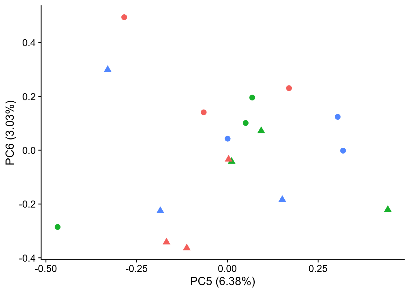
| Version | Author | Date |
|---|---|---|
| e3fbd0f | Anthony Hung | 2021-01-21 |
sessionInfo()R version 3.6.3 (2020-02-29)
Platform: x86_64-apple-darwin15.6.0 (64-bit)
Running under: macOS Catalina 10.15.7
Matrix products: default
BLAS: /Library/Frameworks/R.framework/Versions/3.6/Resources/lib/libRblas.0.dylib
LAPACK: /Library/Frameworks/R.framework/Versions/3.6/Resources/lib/libRlapack.dylib
locale:
[1] en_US.UTF-8/en_US.UTF-8/en_US.UTF-8/C/en_US.UTF-8/en_US.UTF-8
attached base packages:
[1] stats graphics grDevices utils datasets methods base
other attached packages:
[1] ggfortify_0.4.10 dplyr_1.0.2 cowplot_1.1.1 scales_1.1.1
[5] RColorBrewer_1.1-2 edgeR_3.26.8 limma_3.40.6 reshape_0.8.8
[9] ggplot2_3.3.2 gplots_3.0.4
loaded via a namespace (and not attached):
[1] gtools_3.8.2 tidyselect_1.1.0 locfit_1.5-9.4
[4] xfun_0.16 purrr_0.3.4 lattice_0.20-41
[7] colorspace_1.4-1 vctrs_0.3.4 generics_0.0.2
[10] htmltools_0.5.0 yaml_2.2.1 rlang_0.4.7
[13] later_1.1.0.1 pillar_1.4.6 glue_1.4.2
[16] withr_2.2.0 lifecycle_0.2.0 plyr_1.8.6
[19] stringr_1.4.0 munsell_0.5.0 gtable_0.3.0
[22] workflowr_1.6.2 caTools_1.18.0 evaluate_0.14
[25] labeling_0.3 knitr_1.29 httpuv_1.5.4
[28] Rcpp_1.0.5 KernSmooth_2.23-17 promises_1.1.1
[31] backports_1.1.9 gdata_2.18.0 farver_2.0.3
[34] fs_1.5.0 gridExtra_2.3 digest_0.6.25
[37] stringi_1.4.6 grid_3.6.3 rprojroot_1.3-2
[40] tools_3.6.3 bitops_1.0-6 magrittr_1.5
[43] tibble_3.0.3 tidyr_1.1.2 crayon_1.3.4
[46] whisker_0.4 pkgconfig_2.0.3 ellipsis_0.3.1
[49] rmarkdown_2.3 rstudioapi_0.11.0-9000 R6_2.4.1
[52] git2r_0.27.1 compiler_3.6.3